Claude Cohen-Tannoudji - Quantum Mechanics, Volume 3

2 (ii) For a fermion system, the chemical potential has no upper boundary, but the population of an individual state can never exceed 1. If μ is positive, with μ ≫ kBT:– for low values of the energy, the factor 1 is much larger than the exponential term; the population of each individual state is almost equal to 1, its maximum value.– if the energy ei increases to values of the order μ the population decreases and when ei ≫ μ it becomes practically equal to the value predicted by the Boltzmann exponential (27).

Most of the particles occupy, however, the individual states having an energy less or comparable to μ , whose population is close to 1. The fermion system is said to be “degenerate”.

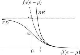
Figure 1 : Quantum distribution functions of Fermi-Dirac (for fermions, lower curve) and of Bose-Einstein (for bosons, upper curve) as a function of the dimensionless variable β ( e – μ ); the dashed line intermediate curve represents the classical Boltzmann distribution e –β (e – μ). In the right-hand side of the figure, corresponding to large negative values of μ, the particle number is small (the low density region) and the two distributions practically join the Boltzmann distribution. The system is said to be non-degenerate, or classical. As μ increases, we reach the central and left hand side of the figure, and the distributions become more and more different, reflecting the increasing gas degeneracy. For bosons, μ cannot be larger than the one-particle ground state energy, assumed to be zero in this case. The divergence observed for μ = 0 corresponds to Bose-Einstein condensation. For fermions, the chemical potential μ can increase without limit, and for all the energy values, the distribution function tends towards 1 (but never exceeding 1 due to the Pauli exclusion principle) .

1 (iii) For a boson system, the chemical potential cannot be larger than the lowest e0 individual energy value, which we assumed to be zero. As μ tends towards zero through negative values and —kBT ≪ μ < 0, the distribution function denominator becomes very small leading to very large populations of the corresponding states. The boson gas is then said to be “degenerate”. On the other hand, for energies of the order or larger than μ, and as was the case for fermions, the boson distribution becomes practically equal to the Boltzmann distribution.

2 (iv) Finally, for situations intermediate between the extreme cases described above, the gas is said to be “partially degenerate”.

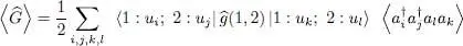
For a two-particle symmetric operator we must use formula (C-16) of Chapter XV, which yields:

(28)

with:

(29)

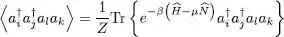
As the exponential operator in the trace is diagonal in the Fock basis states | n 1, .., ni ,.., nj ,..〉, this trace will be non-zero on the double condition that the states i and j associated with the creation operator be exactly the same as the states k and l associated with the annihilation operators, whatever the order. In other words, to get a non-zero trace, we must have either i = l and j = k , or i = k and j = l , or both.

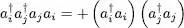
As two fermions cannot occupy the same quantum state, the product is zero if i = j ; we therefore assume i ≠ j which allows, using for ρeq expression (5)(which is a product), to perform independent calculations for the different modes. The case i = l and j = k yields, using the anticommutation relations:

(30)

and the case i = k and j = l yields:

(31)

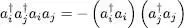
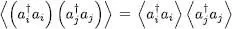
We begin with term (30). As i and j are different, operators and act on different modes, which belong to different factors in the density operator (5). The average value of the product is thus simply the product of the average values:

(32)

(33)

As for the second term (31), it is just the opposite of the first one. Consequently, we finally get:

(34)

The first term on the right-hand side is called the direct term. The second one is the exchange term, and has a minus sign, as expected for fermions.

For bosons, the operators a commute with each other.

If i ≠ j , a calculation, similar to the one we just did, yields:

(35)

which differs in two ways from (34): the result now involves the Bose-Einstein distribution, and the exchange term is positive.

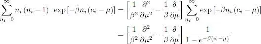
If i = j , only one individual state comes into a new calculation, which we now perform. Using for ρeq expression (5)we get, after summing as in (11)a geometric series:

(36)

The sum appearing in this equation can be written as:

(37)