Claude Cohen-Tannoudji - Quantum Mechanics, Volume 3

(15)

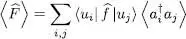
with, when the state of the system is given by the density operator (1):

(16)

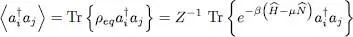
This trace can be computed in the Fock state basis | n 1, .., ni .., nj ,..〉 associated with the eigenstates basis {| uk 〉} of . If i ≠ j , operator destroys a particle in the individual state | uj 〉 and creates another one in the different state | ui 〉; it therefore transforms the Fock state | n 1, .., ni ,.., nj ,..〉 into a different, hence orthogonal, Fock state | n 1,.., ni – 1.., nj + 1,..〉. Operator ρeq then acts on this ket, multiplying it by a constant. Consequently, if i ≠ j , all the diagonal elements of the operator whose trace is taken in (16)are zero; the trace is therefore zero. If i = j , this average value may be computed as for the partition function, since the Fock space has the structure of a tensor product of individual state’s spaces. The trace is the product of the i value contribution by all the other k values contributions. We can thus write, in a general way:

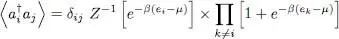
(17)

For i = j , this expression yields the average particle number in the individual state | ui 〉.

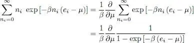
As the occupation number only takes the values 0 and 1, the first bracket in expression (17)is equal to [e –β(ei – μ)]; as for the other modes ( k ≠ i ) contribution, in the second bracket, it has already been computed when we determined the partition function. We therefore obtain:

(18)

Multiplying both the numerator and denominator by 1 + e –β (ei – μ)allows reconstructing the function Z in the numerator, and, after simplification by Z , we get:

(19)

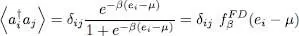
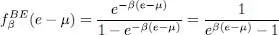
We find again the Fermi-Dirac distribution function (§ 1-b of Complement C XIV):

(20)

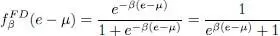
This distribution function gives the average population of each individual state | ui 〉 with energy e ; its value is always less than 1, as expected for fermions.

The average value at thermal equilibrium of any one-particle operator is now readily computed by using (19)in relation (15).

The mode j = i contribution can be expressed as:

(21)

We then get:

(22)

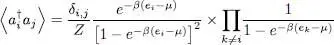
which, using (11), amounts to:

(23)

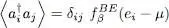
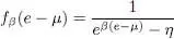
where the Bose-Einstein distribution function is defined as:

(24)

This distribution function gives the average population of the individual state | ui 〉 with energy e . The only constraint of this population, for bosons, is to be positive. The chemical potential is always less than the lowest individual energy ek . In case this energy is zero, μ must always be negative. This avoids any divergence of the function .

Hence for bosons, the average value of any one-particle operator is obtained by inserting (23)into relation (15).

We define the function fβ as equal to either the function for fermions, or the function for bosons. We can write for both cases:

(25)

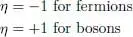
where the number η is defined as:

(26)

We already gave in Complement C XIV( Figure 3) the form of the Fermi-Dirac distribution. Figure 1shows both the variations of this distribution and the Bose-Einstein distribution. For the sake of comparison, it also includes the variations of the classical Boltzmann distribution:

(27)

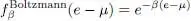
which takes on intermediate values between the two quantum distributions. For a non-interacting gas contained in a box with periodic boundary conditions, the lowest possible energy e is zero and all the others are positive. Exponential e β (ei – μ)is therefore always greater than e –βμ. We are now going to distinguish several cases, starting with the most negative values for the chemical potential.

1 (i) For a negative value of βμ with a modulus large compared to 1 (i.e. for μ ≪ —kBT, which corresponds to the right-hand side of the figure), the exponential in the denominator of (25)is always much larger than 1 (whatever the energy e), and the distribution reduces to the classical Boltzmann distribution (27). Bosons and fermions have practically the same distribution; the gas is said to be “non-degenerate”.