Claude Cohen-Tannoudji - Quantum Mechanics, Volume 3

Figure 2shows the variations of the function as a function of μ , for fixed values of β and the volume .

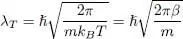
To deal with dimensionless quantities, one often introduces the “thermal wavelength” λ Tas:

(49)

We can then use in the integral of (48)the dimensionless variable:

(50)

and write:

(51)

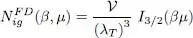
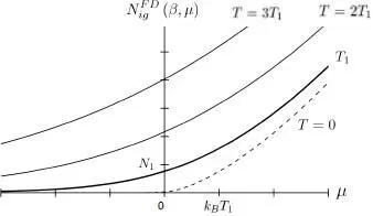
Figure 2: Variations of the particle number for an ideal fermion gas, as a function of the chemical potential μ, and for different fixed temperatures T (β = 1/( kBT ) ). For T = 0 (lower dashed line curve), the particle number is zero for negative values of μ, and proportional to μ3/2 for positive values of μ. For a non-zero temperature T = T 1 (thick line curve), the curve is above the previous one, and never goes to zero. Also shown are the curves obtained for temperatures twice (T = 2 T 1 ) and three times (T = 3 T 1 ) as large. The units chosen for the axes are the thermal energy kBT 1 associated with the thick line curve, and the particle number , where λ T1 is the thermal wavelength at temperature T 1.

Largely negative values of μ correspond to the classical region where the fermion gas is not degenerate; the classical ideal gas equations are then valid to a good approximation. In the region where μ ≫ kBT, the gas is largely degenerate and a Fermi sphere shows up clearly in the momentum space; the total number of particles has only a slight temperature dependence and varies approximately as μ3/2 .

This figure was kindly contributed by Genevieve Tastevin .

with 2 :

(52)

where, in the second equality, we made the change of variable:

(53)

Note that the value of I 3/2only depends on a dimensionless variable, the product βμ .

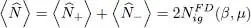
If the particles have a spin 1/2, both contributions and from the two spin states must be added to (46); in the absence of an external magnetic field, the individual particle energies do not depend on their spin direction, and the total particle number is simply doubled:

(54)

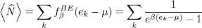
For the sake of simplicity, we shall also start with spinless particles, but including several spin states is fairly straightforward. For bosons, we must use the Bose-Einstein distribution (24)and their average number is therefore:

(55)

We impose periodic boundary conditions in a cubic box of edge length L . The lowest individual energy 3 is ek = 0. Consequently, for expression (55) to be meaningful, μ must be negative or zero:

(56)

Two cases are possible, depending on whether the boson system is condensed or not.

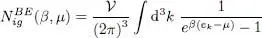
When the parameter μ takes on a sufficiently negative value (much lower than the opposite of the individual energy e 1of the first excited level), the function in the summation (55)is sufficiently regular for the discrete summation to be replaced by an integral (in the limit of large volumes). The average particle number is then written as:

(57)

with:

(58)

Performing the same change of variables as above, this expression becomes:

(59)

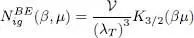
with 4 :

(60)

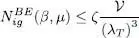
The variations of as a function of μ are shown in Figure 3. Note that the total particle number tends towards a limit as tends towards zero through negative values, where ζ is the number:

(61)

As the function increases with μ , we can write:

(62)

There exists an insurmountable upper limit for the total particle number of a non-condensed ideal Bose gas.

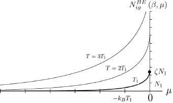
Figure 3: Variations of the total particle number in a non-condensed ideal Bose gas, as a function of μ and for fixed β = 1/( kBT ). The chemical potential is always negative, and the figure shows curves corresponding to several temperatures T = T 1 (thick line), T = 2 T 1 and T = 3 T 1. Units on the axes are the same as in Figure 2: the thermal energy kBT 1 associated with curve T = T 1 , and the particle number , where λ T1 is the thermal wavelength for this same temperature T 1. As the chemical potential tends towards zero, the particle numbers tend towards a finite value. For T = T 1, this value is equal to ζN1 (shown as a dot on the vertical axis), where ζ is given by (61). This figure was kindly contributed by Geneviève Tastevin