Claude Cohen-Tannoudji - Quantum Mechanics, Volume 3
Здесь есть возможность читать онлайн «Claude Cohen-Tannoudji - Quantum Mechanics, Volume 3» — ознакомительный отрывок электронной книги совершенно бесплатно, а после прочтения отрывка купить полную версию. В некоторых случаях можно слушать аудио, скачать через торрент в формате fb2 и присутствует краткое содержание. Жанр: unrecognised, на английском языке. Описание произведения, (предисловие) а так же отзывы посетителей доступны на портале библиотеки ЛибКат.

- Название:Quantum Mechanics, Volume 3
- Автор:
- Жанр:
- Год:неизвестен
- ISBN:нет данных
- Рейтинг книги:5 / 5. Голосов: 1
-
Избранное:Добавить в избранное
- Отзывы:
-
Ваша оценка:
Quantum Mechanics, Volume 3: краткое содержание, описание и аннотация
Предлагаем к чтению аннотацию, описание, краткое содержание или предисловие (зависит от того, что написал сам автор книги «Quantum Mechanics, Volume 3»). Если вы не нашли необходимую информацию о книге — напишите в комментариях, мы постараемся отыскать её.
Quantum Mechanics, Volume 3 — читать онлайн ознакомительный отрывок
Ниже представлен текст книги, разбитый по страницам. Система сохранения места последней прочитанной страницы, позволяет с удобством читать онлайн бесплатно книгу «Quantum Mechanics, Volume 3», без необходимости каждый раз заново искать на чём Вы остановились. Поставьте закладку, и сможете в любой момент перейти на страницу, на которой закончили чтение.
Интервал:
Закладка:
As already mentioned, we shall see in § 4-a that μ is simply the chemical potential.
3. Generalization, Dirac notation
We now go back to the previous line of reasoning, but in a more general case where the bosons may have spins. The variational family is the set of the N -particle state vectors written in (7). The one-body potential may depend on the position r, and, at the same time, act on the spin (particles in a magnetic field gradient, for example).
3-a. Average energy
To compute the average energy value  , we use a basis {| θ k〉} of the individual state space, whose first vector is | θ 1〉 = | θ 〉.
Using relation (B-12) of Chapter XV, we can write the average value  as:
as:
(29) 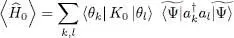
Since  is a Fock state whose only non-zero population is that of the state | θ 1〉, the ket
  is non-zero only if l = 1; it is then orthogonal to
  if k ≠ 1. Consequently, the only term left in the summation corresponds to k = l = 1. As the operator
  multiplies the ket by its population N , we get:
(30) 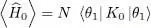
With the same argument, we can write:
(31) 
Using relation (C-16) of Chapter XV, we can express the average value of the interaction energy as 3 :
(32) 
In this case, for the second matrix element to be non-zero, both subscripts m and n must be equal to 1 and the same is true for both subscripts k and l (otherwise the operator will yield a Fock state orthogonal to  ). When all the subscripts are equal to 1, the operator multiplies the ket by N ( N — 1). This leads to:
(33) 
The average interaction energy is therefore simply the product of the number of pairs N ( N —1)/2 that can be formed with N particles and the average interaction energy of a given pair.
We can replace | θ 1〉 by | θ 〉, since they are equal. The variational energy, obtained as the sum of (30), (31)and (33), then reads:
(34) 
3-b. Energy minimization
Consider a variation of | θ 〉:
(35) 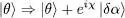
where | δα 〉 is an arbitrary infinitesimal ket of the individual state space, and χ an arbitrary real number. To ensure that the normalization condition (6)is still satisfied, we impose | δα 〉 and | θ 〉 to be orthogonal:
(36) 
so that 〈 θ | θ 〉 remains equal to 1 (to the first order in | δα 〉). Inserting (35)into (34)to obtain the variation  of the variational energy, we get the sum of two terms: the first one comes from the variation of the ket | θ 〉 and is proportional to eiχ the second one comes from the variation of the bra 〈 θ | and is proportional to e–χ . The result has the form:
(37) 
The stationarity condition for  must hold for any arbitrary real value of χ . As before (§ 2-b- α ), it follows that both δc 1and δc 2are zero. Consequently, we can impose the variation to be zero as just the bra 〈 ι | varies (but not the ket | θ 〉), or the opposite.
Varying only the bra, we get the condition:
(38) 
As the interaction operator W 2(1, 2) is symmetric, the last two terms within the bracket in this equation are equal. We get (after simplification by N ):
(39) 
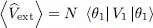
3-c. Gross-Pitaevskii equation
To deal with equation (39), we introduce the Gross-Pitaevskii operator  , defined as a one-particle operator whose matrix elements in an arbitrary basis are {| u i〉} given by:
(40) 
which leads to:
(41) 
Интервал:
Закладка:
Похожие книги на «Quantum Mechanics, Volume 3»
Представляем Вашему вниманию похожие книги на «Quantum Mechanics, Volume 3» списком для выбора. Мы отобрали схожую по названию и смыслу литературу в надежде предоставить читателям больше вариантов отыскать новые, интересные, ещё непрочитанные произведения.


Обсуждение, отзывы о книге «Quantum Mechanics, Volume 3» и просто собственные мнения читателей. Оставьте ваши комментарии, напишите, что Вы думаете о произведении, его смысле или главных героях. Укажите что конкретно понравилось, а что нет, и почему Вы так считаете.