Claude Cohen-Tannoudji - Quantum Mechanics, Volume 3
Здесь есть возможность читать онлайн «Claude Cohen-Tannoudji - Quantum Mechanics, Volume 3» — ознакомительный отрывок электронной книги совершенно бесплатно, а после прочтения отрывка купить полную версию. В некоторых случаях можно слушать аудио, скачать через торрент в формате fb2 и присутствует краткое содержание. Жанр: unrecognised, на английском языке. Описание произведения, (предисловие) а так же отзывы посетителей доступны на портале библиотеки ЛибКат.

- Название:Quantum Mechanics, Volume 3
- Автор:
- Жанр:
- Год:неизвестен
- ISBN:нет данных
- Рейтинг книги:5 / 5. Голосов: 1
-
Избранное:Добавить в избранное
- Отзывы:
-
Ваша оценка:
Quantum Mechanics, Volume 3: краткое содержание, описание и аннотация
Предлагаем к чтению аннотацию, описание, краткое содержание или предисловие (зависит от того, что написал сам автор книги «Quantum Mechanics, Volume 3»). Если вы не нашли необходимую информацию о книге — напишите в комментариях, мы постараемся отыскать её.
Quantum Mechanics, Volume 3 — читать онлайн ознакомительный отрывок
Ниже представлен текст книги, разбитый по страницам. Система сохранения места последней прочитанной страницы, позволяет с удобством читать онлайн бесплатно книгу «Quantum Mechanics, Volume 3», без необходимости каждый раз заново искать на чём Вы остановились. Поставьте закладку, и сможете в любой момент перейти на страницу, на которой закончили чтение.
Интервал:
Закладка:
(B-13) 
Equality (B-11)is then simply written as:
(B-14) 
where  is the occupation number operator in the state | uk 〉 defined in (A-28).
B-3. Examples
A first very simple example is the operator  , already described in (A-29), and corresponding to the total number of particles:
(B-15) 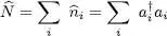
As expected, this operator does not depend on the basis {| ui 〉} chosen to count the particles, as we now show. Using the unitary transformations of operators (A-51)and (A-52), and with the full notation for the creation and annihilation operators to avoid any ambiguity, we get:
(B-16) 
which shows that:
(B-17) 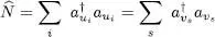
For a spinless particle one can also define the operator corresponding to the probability density at point r 0:
(B-18) 
Relation (B-12)then leads to the “particle local density” (or “single density”) operator:
(B-19) 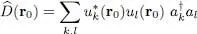
The same procedure as above shows that this operator is independent of the basis {| ui 〉} chosen in the individual states space.
Let us assume now that the chosen basis is formed by the eigenvectors | K i〉 of a particle’s momentum ħ k i, and that the corresponding annihilation operators are noted a ki. The operator associated with the total momentum of the system can be written as:
(B-20) 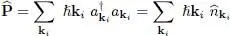
As for the kinetic energy of the particles, its associated operator is expressed as:
(B-21) 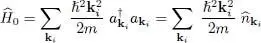
B-4. Single particle density operator
Consider the average value  of a one-particle operator
  in an arbitrary N -particle quantum state. It can be expressed, using relation (B-12), as a function of the average values of operator products
  :
:
(B-22) 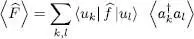
This expression is close to that of the average value of an operator for a physical system composed of a single particle. Remember (Complement E III, § 4-b) that if a system is described by a single particle density operator  , the average value of any operator
  is written as:
(B-23) 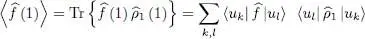
The above two expressions can be made to coincide if, for the system of identical particles, we introduce a “density operator reduced to a single particle”  whose matrix elements are defined by:
(B-24) 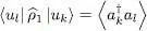
This reduced operator allows computing average values of all the single particle operators as if the system consisted only of a single particle:
(B-25) 
where the trace is taken in the state space of a single particle.
The trace of the reduced density operator thus defined is not equal to unity, but to the average particle number as can be shown using (B-24)and (B-15):
(B-26) 
This normalization convention can be useful. For example, the diagonal matrix element of  in the position representation is simply the average of the particle local density defined in (B-19):
(B-27) 
It is however easy to choose a different normalization for the reduced density operator: its trace can be made equal to 1 by dividing the right-hand side of definition (B-24)by the factor  .
.
C. Two-particle operators
We now extend the previous results to the case of two-particle operators.
C-1. Definition
Consider a physical quantity involving two particles, labeled q and q ′. It is associated with an operator  acting in the state space of these two particles (the tensor product of the two individual state’s spaces). Starting from this binary operator, the easiest way to obtain a symmetric N -particle operator is to sum all the
  over all the particles q and q ′, where the two subscripts q and q ′ range from 1 to N . Note, however, that in this sum all the terms where q = q ′ add up to form a one-particle operator of exactly the same type as those studied in § B-1. Consequently, to obtain a real two-particle operator we shall exclude the terms where q = q ′ and define:
Интервал:
Закладка:
Похожие книги на «Quantum Mechanics, Volume 3»
Представляем Вашему вниманию похожие книги на «Quantum Mechanics, Volume 3» списком для выбора. Мы отобрали схожую по названию и смыслу литературу в надежде предоставить читателям больше вариантов отыскать новые, интересные, ещё непрочитанные произведения.


Обсуждение, отзывы о книге «Quantum Mechanics, Volume 3» и просто собственные мнения читателей. Оставьте ваши комментарии, напишите, что Вы думаете о произведении, его смысле или главных героях. Укажите что конкретно понравилось, а что нет, и почему Вы так считаете.