Claude Cohen-Tannoudji - Quantum Mechanics, Volume 3

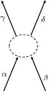
Figure 1: Physical interaction between two identical particles: initially in the states | ukα 〉 and | ukβ 〉 (schematized by the letters α and β), the particles are transferred to the states | ukγ 〉 and | uks 〉 (schematized by the letters γ and δ)

This expression is similar to the average value of an operator for a two-particle system having a density operator :

(C-18)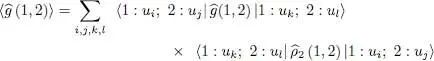

which leads us to define a two-particle reduced density operator :

(C-19)

In this definition we have left out the factor 1/2 of (C-17)since this will lead to a normalization of often more handy: the matrix element of in the position representation yields directly the double density (as well as the field correlation function that we shall study in § B-3-b of Chapter XVI). The trace of is then written:

(C-20)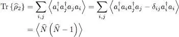

It is obviously possible to divide the right-hand side of the definition of either by the factor 2, or else by the factor if we wish its trace to be equal to 1.

As mentioned in the introduction of this chapter, the equations no longer contain labeled particles, permutations, symmetrizers and antisymmetrizers; the total number of particles N has also disappeared. We may now continue the discussion begun in § D-2 of Chapter XIV concerning the exchange terms, but in a more general way since we no longer specify the total particle number N .

Consider a physical process (schematized in Figure 1) where, in a system of N identical particles, an interaction produces a transfer from the two states | ukα ) and | ukβ 〉 towards the two states | ukγ 〉 and | ukδ 〉; we assume that the four states we are dealing with are different. In the summation over i , j , k , l of (C-16), the only terms involved in this process are those where the bra contains either i = kγ and j = kδ , or the opposite i = kδ and j = kγ ; as for the ket, it must contain either k = kα and l = kβ , or the opposite k = kβ and l = kα . We are then left with four terms:

(C-21)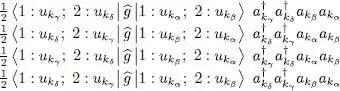

However, since the numbers used to label the particles are dummy variables, the first two matrix elements shown in (C-21)are equal and so are the last two. In addition, the product of creation and annihilation operators obey the following relations, for bosons ( η = 1) as well as for fermions ( η = —1):

(C-22)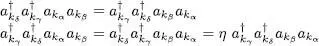

These relations are obvious for bosons since we only commute either creation operators or annihilation operators. For fermions, as we assumed all the states were different, the anticommutation of operators a or of operators a †leads to sign changes; these may cancel out depending on whether the number of anticommutations is even or odd. If we now double the sum of the first and last term of (C-21), we obtain the final contribution to (C-16):

(C-23)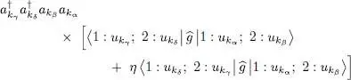

Hence we are left with two terms whose relative sign depends on the nature (bosons or fermions) of the identical particles. They correspond to a different “switching point” for the incoming and outgoing individual states ( Fig. 2).

For bosons, the product of the 4 operators in (C-23)acting on an occupation number ket introduces the square root:

(C-24)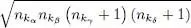

For large occupation numbers, this square root may considerably increase the value of the matrix element. For fermions, however, this amplification effect does not occur. Furthermore, if the direct and exchange matrix elements of are equal, they will cancel each other in (C-23)and the corresponding transition amplitude of this process will be zero.

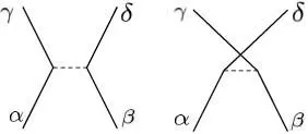
Figure 2: Two diagrams representing schematically the two terms appearing in equation (C-23); they differ by an exchange of the individual states of the exit particles. They correspond, in a manner of speaking, to a different “switching point” for the incoming and outgoing states. The solid lines represent the particles’ free propagation, and the dashed lines their binary interaction .