Abdelkhalak El Hami - Optimizations and Programming

We will first perform Phase I of the simplex algorithm. After adding artificial variables, we obtain the tableau as follows:

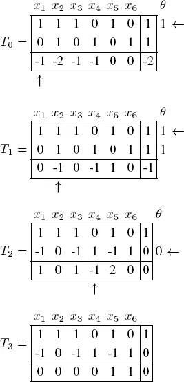
There are no longer any artificial variables in the basis. We have found the optimal tableau of the auxiliary problem, and therefore an admissible basic solution for the initial problem. Since Phase I is now complete, delete the columns corresponding to the artificial variables and compute the reduced costs to obtain the following tableau:

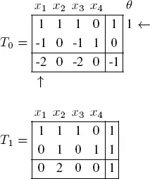
This tableau is optimal. The optimal solution is x 1= 1, x 2= 0, x 3= 0 and x 4= 1, giving an optimal value of z = −1.

Suppose that the current basic admissible solution is degenerate (i.e. at least one basic variable is zero), and let us recall a possible unfavorable scenario that can occur when the simplex algorithm is iterated. Performing a change of basis yields a value for the cost function that is greater than or equal to the previous value. The method is only guaranteed to converge if z * < z 0; in fact, if the previous basic solution is degenerate, it might be the case that z * = z 0.

If this phenomenon occurs multiple times over consecutive iterations, the algorithm can return to a basis that was already considered earlier. In other words, it returns to the same vertex twice. This is called cycling.

Although degeneracy is a frequently encountered phenomenon in linear programming, cycling is not. Some examples have been given in the literature [GAS 75]. Despite the rarity of cycling, it would be desirable to specify a method that avoids it and therefore guarantees that the simplex method will converge. There are several possible choices for a rule that avoids the inconvenience of cycling.

In the past, the most common technique was the so-called method of small perturbations. This method applies an infinitesimal geometric modification to the vector d in order to force it to be expressible as a linear combination of m vectors, with strictly positive coefficients in some basis. Each vertex is then defined as the intersection of n hyperplanes [HIL 90].

More recently, Bland [BLA 77] suggested modifying the rules for choosing the change of basis. Bland’s rule proceeds as follows:

– for the variable entering the basis, choose the smallest index j such that the reduced cost is negative;

– for the variable leaving the basis, if there is equality in θ*, choose the variable with the lowest index.

Earlier, when we solved linear programs graphically, the optimal solutions were on the boundary of the convex set of realizable solutions. If there was a unique optimal solution, it was an extreme point.

Recall the canonical form of a linear program:

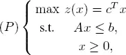
where the matrix A is assumed to be an m × n matrix of rank m (< n ). The standard form is then given by

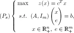
It is possible to show the following result.

Let Γ (respectively, Σ) be the set of feasible solutions of ( P ) (respectively of ( Ps )):

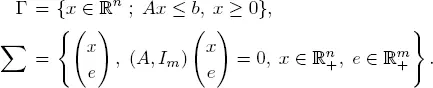
Then Γ and Σ are closed and convex sets.

Recall that the simplex method only uses the basic solutions of ( Ps ). The next theorem tells us that these are in fact the extreme points of Σ.

THEOREM 1.5.– is a basic feasible solution of ( Ps ) if and only if is an extreme point of Σ.

Examples where the solution is not unique show that the optimal solutions lie on the boundary:

THEOREM 1.6.– Every optimal solution of ( P ) (respectively of ( Ps )) belongs to the boundary of Γ (respectively of Σ).

A question presents itself: can there be optimal solutions but no optimal basic feasible solutions? If so, the simplex method, which only considers basic solutions, would not be able to find an optimal solution. The following theorem tells us that this does not happen.

THEOREM 1.7.– If ( Ps ) has an optimal solution, then ( Ps ) has an optimal basic feasible solution.

The simplex algorithm moves along a sequence of vertices of the polyhedron and converges rapidly on average. However, Klee and Minty [KLE 72] found pathological examples where the simplex algorithm visits almost every vertex, which can potentially be an enormous number. The existence of theoretical linear programs that derail the simplex algorithm motivated research to find an algorithm that has polynomial complexity in m and n , even in the worst-case scenarios. Khachian [KHA 79] found the first such algorithm, based on the ellipsoid method from nonlinear optimization. Although it is faster than the simplex method in Minty’s problems, it never succeeded in establishing itself because it tended to be much slower than the simplex algorithm on real problems in practice. Nevertheless, as a mathematical result, it inspired research into interior-point algorithms.

In 1984, Karmarkar [KAR 84] found a new algorithm. The computation time in the worst-case scenario is proportional to n 3.4 L, where L denotes the number of bits required to encode the tableaus A , b and c that define the linear program. The algorithm is too complicated for computations by hand; known as the interior-point algorithm, it enters into the polyhedron itself to converge on the optimal vertex more quickly.

Today, some variants of this algorithm are able to compete with the simplex algorithm. Some software programs already include an interior-point algorithm in addition to the simplex algorithm. On some types of linear programs, interior-point algorithms can be 10 times faster than the simplex algorithm, but nevertheless, there are still many cases where the simplex algorithm is quicker [PRI 11].

EXAMPLE 1.9.– Consider the LP

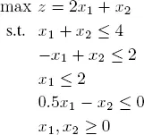
The optimum is x * = (2, 2) T with cost z * = 6. Starting from the interior point x 0= (1, 1) T and without a safety factor, the algorithm performs two iterations: it considers the point x 1= (2, 1.591) T , followed by the point x *.