Efstratios N. Pistikopoulos - Multi-parametric Optimization and Control

1 Cover

2 Wiley Series in

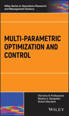
3 Title Page

4 Copyright

5 dedication-page

6 Short Bios of the AuthorsEfstratios N. Pistikopoulos Nikolaos A. Diangelakis Richard Oberdieck

7 Preface

8 Part I Multi‐parametric Optimization 1 Introduction 1.1 Concepts of Optimization 1.2 Concepts of Multi‐parametric Programming 1.3 Polytopes 1.4 Organization of the Book References Notes 2 Multi‐parametric Linear Programming 2.1 Solution Properties 2.2 Degeneracy 2.3 Critical Region Definition 2.4 An Example: Chicago to Topeka 2.5 Literature Review References Notes 3 Multi‐Parametric Quadratic Programming 3.1 Calculation of the Parametric Solution 3.2 Solution Properties 3.3 Chicago to Topeka with Quadratic Distance Cost 3.4 Literature Review References Notes 4 Solution Strategies for mp‐LP and mp‐QP Problems 4.1 General Overview 4.2 The Geometrical Approach 4.3 The Combinatorial Approach 4.4 The Connected‐Graph Approach 4.5 Discussion 4.6 Literature Review References Notes 5 Multi‐parametric Mixed‐integer Linear Programming 5.1 Solution Properties 5.2 Comparing the Solutions from Different mp‐LP Problems 5.3 Multi‐parametric Integer Linear Programming 5.4 Chicago to Topeka Featuring a Purchase Decision 5.5 Literature Review References Notes 6 Multi‐parametric Mixed‐integer Quadratic Programming 6.1 Solution Properties 6.2 Comparing the Solutions from Different mp‐QP Problems 6.3 Envelope of Solutions 6.4 Chicago to Topeka Featuring Quadratic Cost and A Purchase Decision 6.5 Literature Review References Notes 7 Solution Strategies for mp‐MILP and mp‐MIQP Problems 7.1 General Framework 7.2 Global Optimization 7.3 Branch‐and‐Bound 7.4 Exhaustive Enumeration 7.5 The Comparison Procedure 7.6 Discussion 7.7 Literature Review References Notes 8 Solving Multi‐parametric Programming Problems Using MATLAB® 8.1 An Overview over the Functionalities of POP 8.2 Problem Solution 8.3 Problem Generation 8.4 Problem Library 8.5 Graphical User Interface (GUI) 8.6 Computational Performance for Test Sets 8.7 Discussion Acknowledgments References Notes 9 Other Developments in Multi‐parametric Optimization 9.1 Multi‐parametric Nonlinear Programming 9.2 Dynamic Programming via Multi‐parametric Programming 9.3 Multi‐parametric Linear Complementarity Problem 9.4 Inverse Multi‐parametric Programming 9.5 Bilevel Programming Using Multi‐parametric Programming 9.6 Multi‐parametric Multi‐objective Optimization References Notes

9 Part II Multi‐parametric Model Predictive Control 10 Multi‐parametric/Explicit Model Predictive Control10.1 Introduction 10.2 From Transfer Functions to Discrete Time State‐Space Models 10.3 From Discrete Time State‐Space Models to Multi‐parametric Programming 10.4 Explicit LQR – An Example of mp‐MPC 10.5 Size of the Solution and Online Computational Effort References Notes 11 Extensions to Other Classes of Problems 11.1 Hybrid Explicit MPC 11.2 Disturbance Rejection 11.3 Reference Trajectory Tracking 11.4 Moving Horizon Estimation 11.5 Other Developments in Explicit MPC References Notes 12 PAROC: PARametric Optimization and Control12.1 Introduction 12.2 The PAROC Framework 12.3 Case Study: Distillation Column 12.4 Case Study: Simple Buffer Tank12.5 The Tank Example 12.6 Concluding Remarks References Notes

10 AAppendix for the mp‐MPC Chapter 10

11 Appendix for the mp‐MPC Chapter 11 B.1 Matrices for the mp‐QP Problem Corresponding to the Example of Section 11.3.2

12 Index

13 End User License Agreement

1 Chapter 2 Table 2.1 The supply and demand of each plant and market in cases. Table 2.2 The distances between each plant and market in thousands of miles. Table 2.3 The solution of problem (2.20).

2 Chapter 3Table 3.1 The solution of problem (3.14)

3 Chapter 5Table 5.1 The solution of problem (5.16).

4 Chapter 6Table 6.1 The partial solution of problem (6.9). Note that the critical regio...

5 Chapter 7Table 7.1 An overview over the literature on how to solve mp‐MILP and mp‐MIQP...

6 Chapter 10Table 10.1 State expressions as a function of the initial state values and in...Table 10.2 The partial analytical solution of the mp‐MPC problem.Table 10.3 Comparison of optimal unconstrained feedback law (via ) and optima...

7 Chapter 11Table 11.1 The partial analytical solution of the mp‐MPC problem.Table 11.2 The solution of a of the mp‐MPC problem with disturbance.Table 11.3 The partial analytical solution of the mp‐MPC problem.

8 Chapter 12Table 12.1 Interaction of design and control – indicative list.Table 12.2 Integration of scheduling and control – indicative list.Table 12.3 Model approximation of multi‐parametric model‐predictive control –...Table 12.4 Different classes of multi‐parametric programming problems encount...Table 12.5 Parameter values for the distillation column model.Table 12.6 Weight tuning for the mp‐MPC of the tank.

1 Chapter 1 Figure 1.1 A schematic representation of a two‐dimensional polytope . Figure 1.2 A schematic representation of the differences between two polytop... Figure 1.3 A schematic representation of (a) strongly and (b) weakly redunda...

2 Chapter 2 Figure 2.1 The difference between the solution of an LP and an mp‐LP problem... Figure 2.2 A schematic representation of the solution of the mp‐LP problem f... Figure 2.3 A schematic representation of the connected‐graph theorem, (a) fr... Figure 2.4 Primal and dual degeneracy in linear programming. In (a), primal ...

3 Chapter 3Figure 3.1 The difference between the solution of a QP and an mp‐QP problem ...Figure 3.2 A schematic representation of the solution of the mp‐QP problem f...Figure 3.3 A schematic representation of some of the differences between (a)...Figure 3.4 A schematic representation of the connected‐graph theorem, (a) fr...Figure 3.5 The solution to problem 3.14. In (a) the partitioning of the para...

4 Chapter 4Figure 4.1 A schematic representation between the different exploration stra...Figure 4.2 A schematic representation of the failure of the variable step‐si...Figure 4.3 A schematic representation of the branch‐and‐bound algorithm resu...

5 Chapter 5Figure 5.1 The interpretation of mp‐MILP problems as a combination of severa...Figure 5.2 The schematic representation of the example of a comparison proce...Figure 5.3 The detection of the intersection between two critical regions, Figure 5.4 The partitioning of into and based on Eq. (5.7).Figure 5.5 The solution of problem (5.16). In (a) the partitioning of the pa...