Abdelkhalak El Hami - Optimizations and Programming

To do this, we need a second tableau where xJ is replaced by interpreted in the same way as the first. The same linear transformation that allowed us to pass from x to is applied to the columns of A .

The matrix A = ( aij , i = 1, . . . , m , j = 1, . . . , n ) is replaced by Ā = ( āij , i = 1, . . . , m , j = 1, . . . , n ) as follows:

[1.5]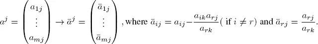

This gives

[1.6]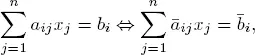

where i , i = 1, . . . , m , are the new basic variables

The last row of the new tableau is computed in the same way:

[1.7]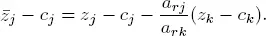

EXAMPLE 1.5.– If we apply the above procedure to our example, we obtain Table 1.2.

Table 1.2. Second simplex tableau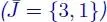

As we saw above, the value of z increases from 0 to 8, but there are still negative values in the last row of the tableau, so we need to perform another change of basis by applying the formulas [1.4] and [1.3] after substituting . This gives:

r = 1, x 3leaves the basis. = {2, 1} is the new basis.

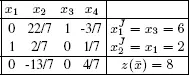
The computation with this new basis is presented in Table 1.3.

Table 1.3. Third simplex tableau

The value of z now increases from 8 to This value is maximal because every value in the final row is non-negative. The optimal solution is therefore This solution is unique because no further change of basis is possible.

EXAMPLE 1.6.– Consider the linear problem:

[1.8]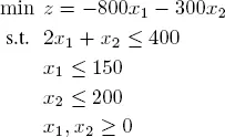

Let us introduce slack variables x 3, x 4and x 5:

[1.9]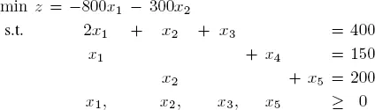

This gives the following initial tableau with the basis ( x 3, x 4, x 5):

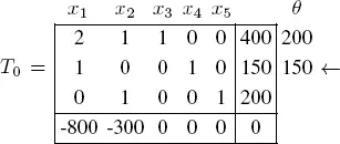
The new basis is ( x 3, x 1, x 5) given as:

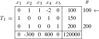
The next basis is ( x 2, x 1, x 5) given as:

Since the reduced costs are all positive, this tableau is optimal. The optimal solution is x 1= 150 and x 2= 100, giving an optimal value of z = −1, 500, 000 for the objective function.

After writing out the first simplex tableau and adding zj = − cj to the last row, there are three possible cases:

1) zj − cj ≥ 0 for j = 1, . . . , n. The basic feasible solution x is already optimal. This optimal solution may or may not be unique;

2) there exists j ∈ {1, . . . , n} such that zj −cj < 0 and aij ≤ 0 for every i ∈ J. In this case, the domain of realizable solutions is unbounded and the problem is ill-posed, since max z(x) = +∞;

3) the usual case: there exists j ∈ {1, . . . , n} such that zj − cj < 0, and there exists i ∈ J such that aij > 0. The change in basis described earlier is now possible and should be performed, possibly several times, until case (1) is reached.

Could the simplex algorithm ever fail to terminate if case (3) leads to a loop? The answer is yes, and examples have been successfully constructed. However, they are very rare in practice.

Let us therefore state two important theorems about the simplex method.

THEOREM 1.3.– Let be a basic realizable solution of ( P ) with respect to a basis J (| J | = m = rank ( A )). Let 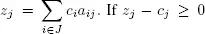for every j = 1, . . . , n , then x is an optimal basic realizable solution.

THEOREM 1.4.– Let be a basic realizable solution of ( P ) with respect to a basis 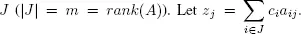Suppose that aij ≤ 0 for every i ∈ J and for every j ∈ {1, . . . , n } such that zj − cj < 0. Then the set { z ( x ), x is a realizable solution} is unbounded.