Abdelkhalak El Hami - Optimizations and Programming

DEFINITION 1.7.– A basic solution of the system of equations Ax = b is obtained by setting n − m variables to zero and solving the system for the remaining p variables. The solution of the system of p equations in m unknowns is assumed to be unique. The n − p variables set to zero are said to be non-basic variables, and the p remaining variables are said to be basic variables. An LP admits, at most, basic solutions. If the basic solution also satisfies the non-negativity constraints, it is said to be a basic feasible solution.

DEFINITION 1.8.– A basic solution is said to be degenerate if at least one basic variable is zero. This type of solution is obtained when the number of lines passing through an extreme point is greater than the number of decision variables. A basic feasible solution whose m basic variables are positive is said to be a non-degenerate basic feasible solution.

REMARK.– Each basic feasible solution corresponds to an extreme point. However, there can be more than one basic feasible solution for the same extreme point. This occurs when the basic feasible solution is degenerate.

REMARK.– The number of basic solutions quickly becomes very large, even in modestly sized models. For example, a model in standard form with 12 constraints and 25 variables can have up to 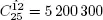basic solutions.

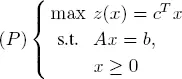
Suppose that we wish to solve

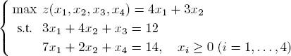
Let c = (4, 3, 0, 0) T , b = (12, 14) T , ( A, I 2) = It is easy to see that x = ( x 1, x 2, x 3, x 4) T = (0, 0, 12, 14) T satisfies the constraints. Thus, x is a basic feasible solution with basis J = {3, 4} (the third and fourth components of x ), whose basic variables are x 3= 12 and x 4= 14.

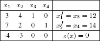
Note that x is not optimal: z ( x ) = c T x = 0. The optimization procedure constructs a sequence of tables, called simplex tableaus. The first tableau summarizes the data c, b, A ′ and the basic variables. The last row is equal to – c T .

Table 1.1. First simplex tableau

Consider the problem

where 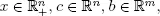and A is an m × n matrix. We may assume without loss of generality that rank A = m < n .

DEFINITION 1.9.– Let A = ( a1 , a2 , . . . , an ) ( where aj is the jth column of A ), and , for J ⊂ {1, 2, . . . , n }, let AJ = { aj , j ∈ J }.

– J ⊂ {1, 2, . . . , n} is a basis of (P) if |J| = m and if rank AJ = rank (aj, j ∈ J) = m;

– let x = (x1, . . . , xn)T ∈ Then xj is a basic variable (respectively, non-basic variable) if j ∈ J (respectively, j ∉ J). We write xJ = (xj, j ∈ J);

– basic feasible solution: x = (x1, . . . , xn)T ∈ such that xj = 0 for j ∉ J and such that Ax = AJ xJ = b.

REMARK.– The advantage of passing from the canonical form to the standard form is that we immediately obtain a basic feasible solution that can be used as a starting point for the simplex algorithm. The basic variables are the slack variables.

Let x be a basic feasible solution of (P). Then

Our goal is to find another feasible basis and a basic feasible solution such that z ( ) > z ( x ) (meaning that is better than x ). The simplex method proceeds by replacing one of the basic variables xr with a non-basic variable xk . We say that

– the variable xr enters the basis J : xr → r = 0;

– the variable xk leaves the basis : xk = 0 → k > 0.

Thus, = ( J − { r }) ∪ { k }. We need rules to choose r and k. These rules are as follows:

– Choose r such that[1.3]

– Choose k such that[1.4]

EXAMPLE 1.4.– Returning to the previous example: J = {3, 4}, c 3= c 4= 0, and so zj = 0 for j = 1, 2, 3, 4. Thus, zj − cj = − cj , j = 1, 2, 3, 4. Hence, k = 1.

To choose r,

Thus, r = 2, x 4leaves the basis, and x 1enters the basis. The new basis is = {3, 1}. We have

Hence, = (2, 0, 6, 0) T and Passing from J = {3, 4} to = {3, 1} increases the value of z to 8, but this value is not yet maximal.

We now apply the transformation x → that increased the value of z. Since the value z ( ) ( > z ( x )) is not necessarily maximal in general, we may need to repeat the steps for choosing r and k several times until we find a basic feasible solution that is also a maximum of z .