Abdelkhalak El Hami - Optimizations and Programming
Здесь есть возможность читать онлайн «Abdelkhalak El Hami - Optimizations and Programming» — ознакомительный отрывок электронной книги совершенно бесплатно, а после прочтения отрывка купить полную версию. В некоторых случаях можно слушать аудио, скачать через торрент в формате fb2 и присутствует краткое содержание. Жанр: unrecognised, на английском языке. Описание произведения, (предисловие) а так же отзывы посетителей доступны на портале библиотеки ЛибКат.
- Название:Optimizations and Programming
- Автор:
- Жанр:
- Год:неизвестен
- ISBN:нет данных
- Рейтинг книги:3 / 5. Голосов: 1
-
Избранное:Добавить в избранное
- Отзывы:
-
Ваша оценка:
Optimizations and Programming: краткое содержание, описание и аннотация
Предлагаем к чтению аннотацию, описание, краткое содержание или предисловие (зависит от того, что написал сам автор книги «Optimizations and Programming»). Если вы не нашли необходимую информацию о книге — напишите в комментариях, мы постараемся отыскать её.
Optimizations and Programming — читать онлайн ознакомительный отрывок
Ниже представлен текст книги, разбитый по страницам. Система сохранения места последней прочитанной страницы, позволяет с удобством читать онлайн бесплатно книгу «Optimizations and Programming», без необходимости каждый раз заново искать на чём Вы остановились. Поставьте закладку, и сможете в любой момент перейти на страницу, на которой закончили чтение.
Интервал:
Закладка:
| P 1 | P 2 | Availability | |
| Equipment | 3 | 9 | 81 |
| Labor | 4 | 5 | 55 |
| Raw materials | 2 | 1 | 20 |
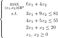
The two products P 1and P 2yield effective profits of 6 dhs and 4 dhs per unit. The goal is to determine which (possibly non-integer) quantities of the products P 1and P 2the factory should produce to maximize the total profit from selling these two products, subject to the availability of the resources.
Let x 1and x 2be the quantities of the products P 1and P 2, respectively.
The LP may be expressed as follows: maximize z ( x 1, x 2) = 6 x 1+ 4 x 2subject to:
– availability of resources:
– positivity of variables: x1, x2 ≥ 0
1.3. Geometry of the linear program
1.3.1. Polyhedra
DEFINITION 1.2.– A polyhedron is a set that can be described as

where A is an m × n matrix and b is a vector in ℝ m. Note that the admissible set of an LP is a polyhedron.
DEFINITION 1.3.– A polyhedron P is said to be bounded if there exists a constant c such that || x || ≤ c for every x ∈ P .
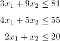
Figure 1.1. Bounded polyhedron (left) and unbounded polyhedron (right). For a color version of this figure, see www.iste.co.uk/radi/optimizations.zip
DEFINITION 1.4.– Let a be a non-zero vector of ℝ n, and let b be a scalar.
– The set {x ∈ ℝn|aTx = b} is said to be a hyperplane.
– The set {x ∈ ℝn|aTx ≥ b} is said to be a half-space.
Note that a hyperplane is the boundary of the corresponding half-space and the vector a is perpendicular to the hyperplane that it defines [TEG 12].
1.3.2. Extreme points and vertices
Let P be a polyhedron and x * ∈ P . The point x * is an extreme point if and only if x * is a vertex and x * is a basic admissible solution.
DEFINITION 1.5.– Let P be a polyhedron. A vector x ∈ P is an extreme point of P if it cannot be expressed as a convex combination of two other points of P .
DEFINITION 1.6.– Let P be a polyhedron. A vector x ∈ P is a vertex of P if there exists c such that

for every y in P not equal to x.
THEOREM 1.2.– In linear programming, if the admissible domain is neither empty nor the whole of ℝ n , it is a convex polytope with finitely many vertices that can either be bounded or unbounded. If an extreme point exists, it is attained at one of the vertices of the polytope. A point in the interior of the domain is never an extreme point if f ≠ 0. If the polytope is bounded, f attains both a minimum and a maximum on it.
This theorem gives us a graphical solving method.
1.4. Graphical solving of a linear program
The graphical method works by plotting lines and searching for a solution as follows:
– identify the admissible domain;
– identify the contours;
– contours perpendicular to the vector c, and therefore mutually parallel;
– each value of z is associated with a contour;
– the value of z increases in the direction of c.
EXAMPLE 1.2.– Consider, again, the example from earlier. Its mathematical model is defined by the following linear program:
The intersection of the half-planes determined by the lines corresponding to each constraint represents the set of solutions that satisfy the constraints (shaded area). The direction of the cost function is given by

This gives us the optimal solution  by sliding the line with this direction upwards, while keeping it parallel, until its intersection with the y-axis is maximal. Graphical solutions are of course only applicable with programs of, at most, three variables (see Figure 1.2).
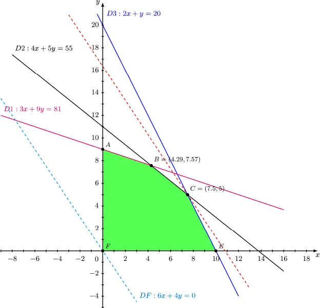
Figure 1.2. Graphical solution. For a color version of this figure, see www.iste.co.uk/radi/optimizations.zip
EXAMPLE 1.3.– Consider the linear program:
[1.2] 
The graphical solution is shown in Figure 1.3. We have z * = −2, with 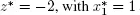 and
and 
Figure 1.3. Graphical solution with isoprofit lines. For a color version of this figure, see www.iste.co.uk/radi/optimizations.zip
1.5. Simplex algorithm
If a linear programming problem in standard form has an optimal solution, then a basic admissible solution that is optimal exists. The simplex algorithm is an algorithm for solving linear optimization problems. Introduced by George Dantzig in 1947, it was probably the earliest algorithm for minimizing functions on sets defined by inequalities. The algorithm moves from one basic admissible solution to the next while reducing the cost.
The idea of the method is as follows:
– Let x0 be a basic admissible solution.
– For k = 0, . . . , find an adjacent basic admissible solution xk+1 such that .
– Until no adjacent basic admissible solution improves the objective.
This gives a local minimum, which is in fact a global minimum in linear programming.
1.5.1. Basic solutions and basic feasible solutions
Consider a system of m linear equations Ax = b with n variables ( m ≤ n ).
Читать дальшеИнтервал:
Закладка:
Похожие книги на «Optimizations and Programming»
Представляем Вашему вниманию похожие книги на «Optimizations and Programming» списком для выбора. Мы отобрали схожую по названию и смыслу литературу в надежде предоставить читателям больше вариантов отыскать новые, интересные, ещё непрочитанные произведения.


Обсуждение, отзывы о книге «Optimizations and Programming» и просто собственные мнения читателей. Оставьте ваши комментарии, напишите, что Вы думаете о произведении, его смысле или главных героях. Укажите что конкретно понравилось, а что нет, и почему Вы так считаете.