Abdelkhalak El Hami - Optimizations and Programming
Здесь есть возможность читать онлайн «Abdelkhalak El Hami - Optimizations and Programming» — ознакомительный отрывок электронной книги совершенно бесплатно, а после прочтения отрывка купить полную версию. В некоторых случаях можно слушать аудио, скачать через торрент в формате fb2 и присутствует краткое содержание. Жанр: unrecognised, на английском языке. Описание произведения, (предисловие) а так же отзывы посетителей доступны на портале библиотеки ЛибКат.
- Название:Optimizations and Programming
- Автор:
- Жанр:
- Год:неизвестен
- ISBN:нет данных
- Рейтинг книги:3 / 5. Голосов: 1
-
Избранное:Добавить в избранное
- Отзывы:
-
Ваша оценка:
Optimizations and Programming: краткое содержание, описание и аннотация
Предлагаем к чтению аннотацию, описание, краткое содержание или предисловие (зависит от того, что написал сам автор книги «Optimizations and Programming»). Если вы не нашли необходимую информацию о книге — напишите в комментариях, мы постараемся отыскать её.
Optimizations and Programming — читать онлайн ознакомительный отрывок
Ниже представлен текст книги, разбитый по страницам. Система сохранения места последней прочитанной страницы, позволяет с удобством читать онлайн бесплатно книгу «Optimizations and Programming», без необходимости каждый раз заново искать на чём Вы остановились. Поставьте закладку, и сможете в любой момент перейти на страницу, на которой закончили чтение.
Интервал:
Закладка:
Let x be the number of large automobiles manufactured, y the number of small automobiles manufactured and z the resulting turnover. The problem can therefore be expressed in the form:
[1.21] 
1.11.1. Optimal solution
It is relatively easy to find a graphical solution for systems like this with only two variables. This allows us to find the optimal solution x = 200 and y = 200, which corresponds to z = 5, 200, 000. In this particular example, the optimal solution is unique, corresponding to a vertex of the region bounded by the constraints.
1.11.2. Sensitivity to variation in stock
Let us observe how the solution of the problem evolves when some of the starting data is modified, for example by increasing the stock of rubber or steel. Suppose that 700 units of steel are in stock instead of 600. The problem now becomes:
[1.22] 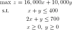
By solving graphically again, we find that the optimal solution is now x = 300 and y = 100, giving z = 5, 800, 000. In other words, increasing the available steel by 100 units increases the turnover by 600,000 euros. We say that the marginal price of a unit of steel is 6,000 euros.
If the amount of steel in stock is increased to 800, the optimal solution becomes x = 400 and y = 0, and the turnover becomes z = 6, 400, 000. Increasing the steel in stock beyond 800 without also changing the rubber in stock no longer affects the optimal solution, because y is constrained to remain positive.
Suppose now that the steel in stock remains fixed at 600, but the rubber in stock is increased by 400 to 500. The new problem is
[1.23] 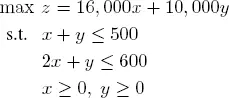
Graphical solving shows that the optimal solution is now given by x = 100 and y = 400, which corresponds to z = 5, 600, 000. In other words, increasing the rubber by 100 units changes the turnover by 400,000 euros. We say that the marginal price of a unit of rubber is 4,000 euros.
If the rubber in stock is increased to 600, the optimal solution becomes x = 0 and y = 600, and the turnover becomes z = 6, 000, 000. Increasing the amount of rubber in stock beyond 600, without also increasing the amount of steel in stock, no longer affects the optimal solution because x is constrained to remain positive.
1.11.3. Dual problem of the competitor
Suppose now that the automobile manufacturer has a competitor who offers to repurchase all raw materials in stock to fulfill a large number of orders. The competitor must offer a certain price (assumed to be constant and denoted u ) per unit of rubber and another price (denoted v ) per unit of steel. For the offer to be accepted, the price paid by the competitor must at least be equal to the turnover that the manufacturer could achieve by manufacturing automobiles itself. The competitor’s problem can therefore be written as
[1.24] 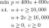
Graphical analysis finds the optimal solution u = 4, 000 and v = 6, 000, which corresponds to a global price of p = 5, 200, 000. Observe (and we will see later that this is no coincidence) that the optimal solution of the competitor’s problem (the dual problem to the manufacturer’s primal problem) coincides with the marginal prices of the manufacturer’s problem, and the minimum price that the competitor can offer is equal to the manufacturer’s maximum turnover.
1.12. Using Matlab
Matlab offers the linprog solver for optimizing LPs. The linprog solver takes the following input arguments:
– f: the objective function;
– A: the matrix of inequality constraints;
– b: the right-hand side of the inequality constraints;
– Aeq: the matrix of equality constraints;
– beq: the right-hand side of the equality constraints;
– lb: the vector of lower bounds of the decision variables;
– ub: the vector of upper bounds of the decision variables;
– x0: the starting point of x, only used for the active-set algorithm;
– options : options created with “optimoptions”.
All linprog arguments use the following options, defined via the “optimoptions” input:
– Algorithm: the following algorithms can be used:1) “interior-point” (default);2) “dual-simplex”;3) “active-set”;4) “simplex”.
– LargeScale: the “interior-point” algorithm is used when this option is set to “on” (default) and the primal simplex algorithm is used when it is set to “off”.
– TolCon: the feasibility tolerance for constraints. The default value is 1e-4. It takes scalar values from 1e-10 to 1e-3 (only available for the dual simplex algorithm).
The output arguments of the linprog solver are as follows:
– fval: the value of the objective function at the solution x;
– x: the solution found by the solver. If exitflag > 0, then x is a solution; if not, x is the value of the variables when the solver terminated prematurely;
– exitflag: the reason why the algorithm terminated:- 1: the solver converged to the solution x;- 0: the number of iterations exceeded the “MaxIter option”;- 2: no feasible point was found;- 3: the LP problem is not bounded;- 4: a NaN value was encountered when executing the algorithm;- 5: the primal and dual problems are infeasible;- 7: the search direction became too small and no other progress was observed.
The following list specifies the various syntaxes that can be used to call the linprog solver:
– x = linprog(f, A, b): solves min fT x such that Ax ≤ b (used when there are only equality constraints);
– x = linprog(f, A, b, Aeq, beq): solves the problem with the equality constraints Aeqx = beq. Set A=[ ] and b=[ ] if no inequalities exist;
– x = linprog(f, A, b, Aeq, beq, lb, ub): defines a set of lower and upper bounds on the design variables, x, so that the solution is always in the range lb ≤ x ≤ ub. Set Aeq=[ ] and beq=[ ] if no equalities exist;
– x = linprog(f, A, b, Aeq, beq, lb, ub, x0): defines the starting point at x0 (only used for the active-set algorithm);
– x = linprog(f, A, b, Aeq, beq, lb, ub, x0, options): minimizes with the specified options;
– [x, fval] = linprog(...): returns the value of the objective function at the solution x;
– [x, fval, exitflag] = linprog(...): returns a value exitflag that describes the exit condition;
– [x, fval, exitflag, output] = linprog(...): returns a structure output that contains information about the optimization process;
– [x, fval, exitflag, output, lambda] = linprog(...): returns a structure output whose fields contain the Lagrange multipliers λ at the solution x.
EXAMPLE 1.14.– Consider the linear program:
[1.25] 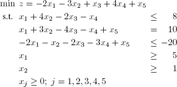
Интервал:
Закладка:
Похожие книги на «Optimizations and Programming»
Представляем Вашему вниманию похожие книги на «Optimizations and Programming» списком для выбора. Мы отобрали схожую по названию и смыслу литературу в надежде предоставить читателям больше вариантов отыскать новые, интересные, ещё непрочитанные произведения.


Обсуждение, отзывы о книге «Optimizations and Programming» и просто собственные мнения читателей. Оставьте ваши комментарии, напишите, что Вы думаете о произведении, его смысле или главных героях. Укажите что конкретно понравилось, а что нет, и почему Вы так считаете.