Abdelkhalak El Hami - Optimizations and Programming

Let xB be the basic variables of the solution. Our goal is to determine a condition that guarantees that the basis B will remain optimal. In fact, this is easy. The vector b only appears in the optimality condition [1.16]. Therefore, the basic variables xB remain optimal for the modified problem if

[1.17]

EXAMPLE 1.12.– Consider the LP:

[1.18]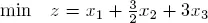

[1.19]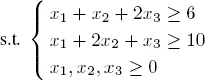

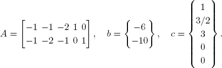
In matrix form with slack variables, this can be written as:

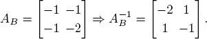
Suppose that the optimal basis is B = { x 1, x 2}. Then

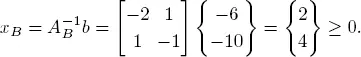
Compute xB :

Compute the reduced costs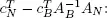

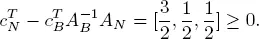
The solution xB = (2, 4) T is therefore optimal, i.e. x = (2, 4, 0, 0, 0) T .

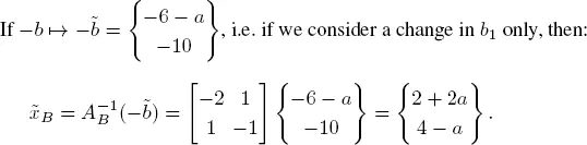
We will have if and only if

2 + 2 a ≥ 0 and 4 − a ≥ 0.

This gives an interval for the parameter b 1: −1 ≤ a ≤ 4.

What is the interval for b 2?

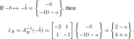
We will have B ≥ 0 if and only if

2 − a ≥ 0 and 4 + a ≥ 0.

This gives the interval for the parameter b 2: −4 ≤ a ≤ 2.

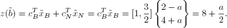
What is the effect on the minimum value of the objective function?

The effect is:

Next, let us find a condition that guarantees that the basis B will remain optimal under First, observe that the solution remains unchanged. However, the simplex tableau might no longer be optimal. To keep it optimal, we must impose the stability condition

[1.20]

In general, let us determine the effect of modifying a single variable xi :

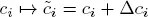
There are two cases to analyze depending on whether xi is a basic or non-basic variable.

Write ei for the canonical basis vector of ℝ n , i.e. ei = (0, 0, . . . , 1, 0, . . . , 0) T with 1 at position i . Then:

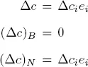
The i th component of the vector 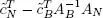is

where the ri are the components of the final row of the simplex tableau. In other words, we have all the information that we need to compute the stability intervals of the coefficients ci .

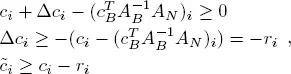
EXAMPLE 1.13.– Again, consider the previous example. The final simplex tableau is:

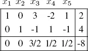
The last row gives us the vector of reduced costs 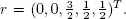The basic variables are B = { x 1, x 2}, and the non-basic variables are N = { x 3, x 4, x 5}. The objective function is of the form z = c 1 x 1+ c 2 x 2+ c 3 x 3with 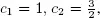and c 3= 3. It does not make sense to perturb the coefficients c 4and c 5. Accordingly, we can only perturb x 3. Let us compute the stability interval around c 3associated with the non-basic variable x 3. The stability condition is

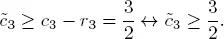
The optimal solution x = (2, 4, 0, 0, 0) T is the same for every value Furthermore, the value of the objective function ( z = 8) remains unchanged because the variable is non-basic.

Consider the problem of an automobile manufacturer that offers two models for sale, a small automobile and a large automobile. Suppose that there is sufficient demand that the manufacturer is certain to sell whatever is produced at the current sales price of 16,000 euros for large automobiles, and 10,000 euros for small ones. The manufacturer’s only problem is the limited supply of two raw materials, rubber and steel. Manufacturing a small automobile requires one unit of rubber and one unit of steel, whereas manufacturing a large automobile requires one unit of rubber and two units of steel. If the manufacturer has 400 units of rubber and 600 units of steel in stock, how many small and large vehicles should be produced from this inventory to maximize the turnover?