Abdelkhalak El Hami - Optimizations and Programming
Здесь есть возможность читать онлайн «Abdelkhalak El Hami - Optimizations and Programming» — ознакомительный отрывок электронной книги совершенно бесплатно, а после прочтения отрывка купить полную версию. В некоторых случаях можно слушать аудио, скачать через торрент в формате fb2 и присутствует краткое содержание. Жанр: unrecognised, на английском языке. Описание произведения, (предисловие) а так же отзывы посетителей доступны на портале библиотеки ЛибКат.
- Название:Optimizations and Programming
- Автор:
- Жанр:
- Год:неизвестен
- ISBN:нет данных
- Рейтинг книги:3 / 5. Голосов: 1
-
Избранное:Добавить в избранное
- Отзывы:
-
Ваша оценка:
Optimizations and Programming: краткое содержание, описание и аннотация
Предлагаем к чтению аннотацию, описание, краткое содержание или предисловие (зависит от того, что написал сам автор книги «Optimizations and Programming»). Если вы не нашли необходимую информацию о книге — напишите в комментариях, мы постараемся отыскать её.
Optimizations and Programming — читать онлайн ознакомительный отрывок
Ниже представлен текст книги, разбитый по страницам. Система сохранения места последней прочитанной страницы, позволяет с удобством читать онлайн бесплатно книгу «Optimizations and Programming», без необходимости каждый раз заново искать на чём Вы остановились. Поставьте закладку, и сможете в любой момент перейти на страницу, на которой закончили чтение.
Интервал:
Закладка:
This relaxation often produces a very good relaxation value, far better than continuous relaxation.
Consider the following LP:
[1.11] 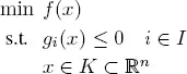
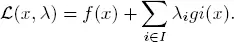
To each constraint i ∈ I , we assign a real number λ i≥ 0 called the Lagrange multiplier. We also define the vector λ = (λ i, 0 i ∈ I ). The Lagrangian function is then defined as
This function has the two vector arguments x and λ and takes values in ℝ. Suppose that the PL is such that the problem min x∈S  ( x , λ) has an optimal solution for every λ ≥ 0.
More details are given in Chapter 7. Now consider the following LP [FLE 10]:
[1.12] 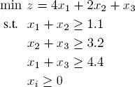
We obtain the optimal solution (0, 1.1, 4.4) T , which gives the optimal cost as z * = 6.6.
By relaxing the third constraint ( x 1+ x 2≥ 4.4) and keeping the integrality constraints on the variables xi , we obtain the following LP by adding the expression λ(4.4 − x 1− x 3) to the objective function, where λ is the Lagrangian relaxation coefficient, which is updated at each iteration of the method:
[1.13] 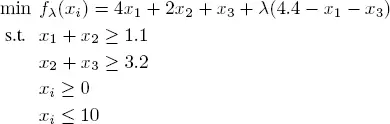
The last constraint is added to bound the variables xi . This guarantees that the problem is bounded for every λ > 0. The coefficient λ is updated as follows: λ k+1= max 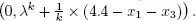 It can be shown that λ tends to 1 and z tends to 8.4.
1.10. Postoptimal analysis
Consider the LP:
[1.14] 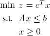
We will now perform a postoptimal analysis of the optimal solution in terms of the problem data, also known as a sensitivity analysis. In other words, how does the solution or the objective function vary if we modify one of the entries of the vectors c or b , or the matrix A ?
To conduct a postoptimal analysis, we need to be able to express the solution of the simplex algorithm in terms of the initial problem data instead of simplex tableaus, which change at each iteration.
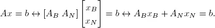
As always, we introduce slack variables to the problem [1.14], writing A for the resulting matrix of size m × ( m + n ). We also assume that the basic variables B of the optimal solution xB are known. This information can be read off from the final tableau of the simplex algorithm, which is why this procedure is called postoptimal analysis.
Let B = { x j1, x j2, . . . , xjm } be the list of basic variables, and let N be its complement with respect to the index set {1, 2, . . . , m + n }. For example, if m = n = 3 and B = { x 1, x 5, x 2}, then N = { x 3, x 4, x 6}. Based on the sets B and N , we can extract the following submatrices of A :
– AB is the submatrix formed by the columns corresponding to the variables of B. We take them in the order specified by B.
– AN is the submatrix formed by the columns corresponding to the variables of N in the order specified by N.
EXAMPLE 1.11.– Consider the problem
[1.15] 
The matrix system Ax = b with slack variables is given as
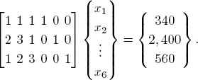
The final tableau of the simplex algorithm is written as
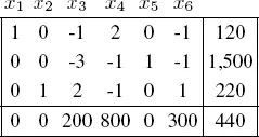
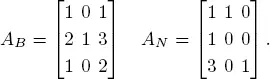
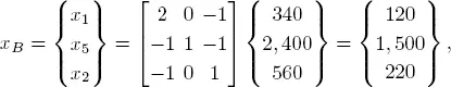
We therefore indeed have B = { x 1, x 5, x 2} and N = { x 3, x 4, x 6}. The submatrices AB and AN can be written as:
Using a block partition based on the index sets B and N , we can write
The solution  can be computed algebraically. The matrix AB is invertible because B is a basis. The optimal solution is given by the formula
  since the non-basic variables must be zero, i.e. xN = 0. In our example, we have
which is the correct optimal solution according to the final simplex tableau. The other columns of the final tableau correspond to
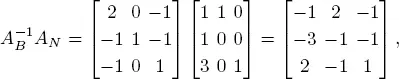
which are indeed the columns that correspond to N = { x 3, x 4, x 6}.
1.10.1. Effect of modifying b
Let us analyze the effect of modifying the vector b . In other words, we shall study the behavior of the solution of the modified problem when b is replaced by  = b +Δ b .
[1.16] 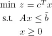
Интервал:
Закладка:
Похожие книги на «Optimizations and Programming»
Представляем Вашему вниманию похожие книги на «Optimizations and Programming» списком для выбора. Мы отобрали схожую по названию и смыслу литературу в надежде предоставить читателям больше вариантов отыскать новые, интересные, ещё непрочитанные произведения.


Обсуждение, отзывы о книге «Optimizations and Programming» и просто собственные мнения читателей. Оставьте ваши комментарии, напишите, что Вы думаете о произведении, его смысле или главных героях. Укажите что конкретно понравилось, а что нет, и почему Вы так считаете.