Barna Szabó - Finite Element Analysis

and the exact value of the QoI is

(1.110)

Subtracting eq. (1.109)from eq. (1.110)we get

(1.111)

We define a function such that

(1.112)

This operation projects onto the space . Letting 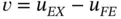we get:

We will write this as

(1.113)

Next we define such that

(1.114)

This operation projects onto the space . By Galerkin's orthogonality condition (see Theorem 1.3) we have

Therefore, letting , we write eq. (1.113)as

(1.115)

and we can write eq. (1.111)as

(1.116)

Therefore the error in the extracted data is

(1.117)

where we used the Schwarz inequality, see Section A.3in the appendix.

The function made it possible to write the error in the QoI in this form. It does not have to be computed.

Inequality (1.117)serves to explain why the error in the extracted data can converge to zero faster than the error in energy norm: If is of comparable magnitude to then the error in the extracted data is of comparable magnitude to the error in the strain energy, that is, the error in energy norm squared. But, as seen in Example 1.9, where w was much smoother than , it can be much smaller. In the exceptional case when the extraction function is Green's function, the error is zero.

In an ideal discretization the error (in energy norm) associated with each element would be the same. This ideal discretization can be approximated by automated adaptive methods in which the discretization is modified based on feedback information from previously obtained finite element solutions. Alternatively, based on a general understanding of the relationship between regularity and discretization, and understanding the strengths and limitations of the software tools available to them, analysts can formulate very efficient discretization schemes.

When the solution is smooth then the most efficient finite element discretization scheme is uniform mesh and high polynomial degree. However, all implementations of finite element analysis software have limitations on how high the polynomial degree is allowed to be and therefore it may not be possible to increase the polynomial degree sufficiently to achieve the desired accuracy. In such cases the mesh has to be refined. Uniform refinement may not be optimal in all cases, however. Consider, for example, the following problem:

(1.118)

where , and f is a smooth function. Intuitively, when is small then the solution will be close to however, because of the boundary condition , has to be satisfied, the function will change sharply over some interval .

Letting and the exact solution of this problem is