Barna Szabó - Finite Element Analysis

The first term of the bilinear form in eq. (1.43)is computed as a sum of integrals over the elements

(1.62)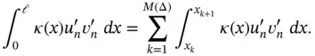

We will be concerned with the evaluation of the integral on the k th element:

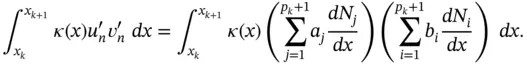
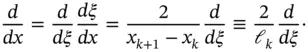
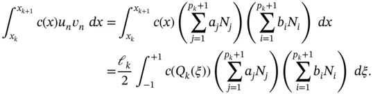
The shape functions Ni are defined on the standard domain . Referring to the mapping function given by eq. (1.60), we have

(1.63)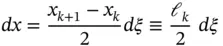

where 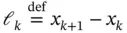is the length of the k th element. Also,

Therefore

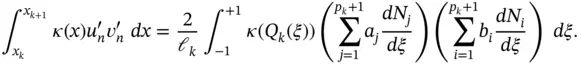
We define

(1.64)

and write

(1.65)

The terms of the stiffness matrix depend on the the mapping, the definition of the shape functions and the function . The matrix is called the element stiffness matrix. Observe that that is, is symmetric. This follows directly from the symmetry of and the fact that the same basis functions are used for un and vn .

In the finite element method the integrals are evaluated by numerical methods. Numerical integration is discussed in Appendix E. In the important special case when is constant on Ik , it is possible to compute once and for all. This is illustrated by the following example.

Example 1.3When is constant on Ik and the Legendre shape functions are used then, with the exception of the first two rows and columns, the element stiffness matrix is perfectly diagonal:

(1.66)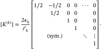

Exercise 1.8Assume that is constant on Ik . Using the Lagrange shape functions displayed in Fig. 1.3for , compute and in terms of κk and ℓk .

The second term of the bilinear form is also computed as a sum of integrals over the elements:

(1.67)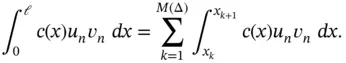

We will be concerned with evaluation of the integral

Defining:

(1.68)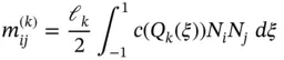

the following expression is obtained:

(1.69)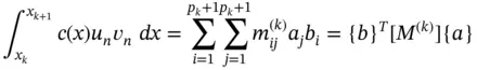

where 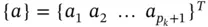, 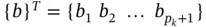and

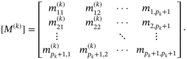
The terms of the coefficient matrix are computable from the mapping, the definition of the shape functions and the function . The matrix is called the element‐level Gram matrix 13 or the element‐level mass matrix. Observe that is symmetric. In the important special case where is constant on Ik it is possible to compute once and for all. This is illustrated by the following example.