Barna Szabó - Finite Element Analysis

The choice of basis functions is guided by considerations of implementation, keeping the condition number of the coefficient matrices small, and personal preferences. For the symmetric positive‐definite matrices considered here the condition number C is the largest eigenvalue divided by the smallest. The number of digits lost in solving a linear problem is roughly equal to . Characterizing the condition number as being large or small should be understood in this context. In the finite element method the condition number depends on the choice of the basis functions and the mesh.

The standard polynomial basis functions, called shape functions, can be defined in various ways. We will consider shape functions based on Lagrange polynomials and Legendre 12 polynomials. We will use the same notation for both types of shape function.

Lagrange shape functions of degree p are constructed by partitioning into p sub‐intervals. The length of the sub‐intervals is typically but the lengths may vary. The node points are , and 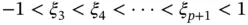. The i th shape function is unity in the i th node point and is zero in the other node points:

(1.50)

These shape functions have the following important properties:

(1.51)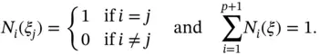

For example, for the equally spaced node points are , , . The corresponding Lagrange shape functions are illustrated in Fig. 1.3.

Exercise 1.5Sketch the Lagrange shape functions for .

For we have

(1.52)

For we define the shape functions as follows:

(1.53)

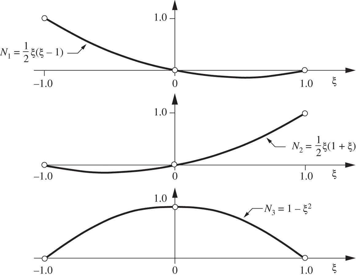
Figure 1.3 Lagrange shape functions in one dimension, .

where are the Legendre polynomials. The definition of Legendre polynomials is given in Appendix D. These shape functions have the following important properties:

1 Orthogonality. For :(1.54) This property follows directly from the orthogonality of Legendre polynomials, see eq. (D.13) in the appendix.

2 The set of shape functions of degree p is a subset of the set of shape functions of degree . Shape functions that have this property are called hierarchic shape functions.

3 These shape functions vanish at the endpoints of : for .

The first five hierarchic shape functions are shown in Fig. 1.4. Observe that all roots lie in . Additional shape functions, up to , can be found in the appendix, Section D.1.

Exercise 1.6Show that for the hierarchic shape functions, defined by eq. (1.53), for .

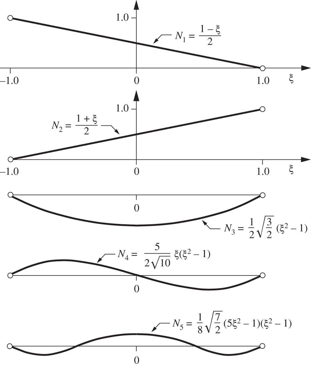
Figure 1.4 Legendre shape functions in one dimension, .

Exercise 1.7Show that the hierarchic shape functions defined by eq. (1.53)can be written in the form:

(1.55)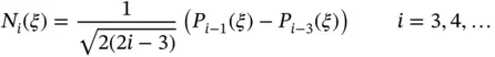

Hint: note that for all n and use equations (D.10) and (D.12) in Appendix D.

We are now in a position to provide a precise definition of finite element spaces in one dimension.

The domain 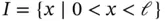is partitioned into M non‐overlapping intervals called finite elements. A partition, called finite element mesh, is denoted by . Thus . The boundary points of the elements are the node points. The coordinates of the node points, sorted in ascending order, are denoted by xi , ( ) where and . The k th element Ik has the boundary points xk and , that is, .