Barna Szabó - Finite Element Analysis
Здесь есть возможность читать онлайн «Barna Szabó - Finite Element Analysis» — ознакомительный отрывок электронной книги совершенно бесплатно, а после прочтения отрывка купить полную версию. В некоторых случаях можно слушать аудио, скачать через торрент в формате fb2 и присутствует краткое содержание. Жанр: unrecognised, на английском языке. Описание произведения, (предисловие) а так же отзывы посетителей доступны на портале библиотеки ЛибКат.
- Название:Finite Element Analysis
- Автор:
- Жанр:
- Год:неизвестен
- ISBN:нет данных
- Рейтинг книги:5 / 5. Голосов: 1
-
Избранное:Добавить в избранное
- Отзывы:
-
Ваша оценка:
Finite Element Analysis: краткое содержание, описание и аннотация
Предлагаем к чтению аннотацию, описание, краткое содержание или предисловие (зависит от того, что написал сам автор книги «Finite Element Analysis»). Если вы не нашли необходимую информацию о книге — напишите в комментариях, мы постараемся отыскать её.
Finite Element Analysis — читать онлайн ознакомительный отрывок
Ниже представлен текст книги, разбитый по страницам. Система сохранения места последней прочитанной страницы, позволяет с удобством читать онлайн бесплатно книгу «Finite Element Analysis», без необходимости каждый раз заново искать на чём Вы остановились. Поставьте закладку, и сможете в любой момент перейти на страницу, на которой закончили чтение.
Интервал:
Закладка:
Exercise 1.12Let
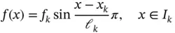
where fk is a constant. Compute  numerically in terms of fk and ℓk using 3, 4 and 5 Gauss points. See Appendix E. Use the Legendre basis functions.
Exercise 1.13Assume that  is a linear function on I . Using the Lagrange shape functions for
  , compute
  .
.
1.3.5 Assembly
Having computed the coefficient matrices and right hand side vectors for each element, it is necessary to form the coefficient matrix and right hand side vector for the entire mesh. This process, called assembly, executes the summation in equations (1.62), (1.67)and (1.73). The local and global numbering of variables is reconciled in the assembly process. The algorithm is illustrated by the following example.
Example 1.6Consider the three‐element mesh shown in Fig. 1.5. The polynomial degrees  ,
,  ,
,  are assigned to elements 1, 2, 3 respectively. The basis functions shown in Fig. 1.5are composed of the mapped Legendre shape functions. For instance, the basis function
  is composed of the mapped shape function N 2from element 1 and the mapped shape function N 1from element 2. This basis function is zero over element 3. Basis function
  is the mapped shape function N 3from element 3. This basis function is zero over elements 1 and 2.
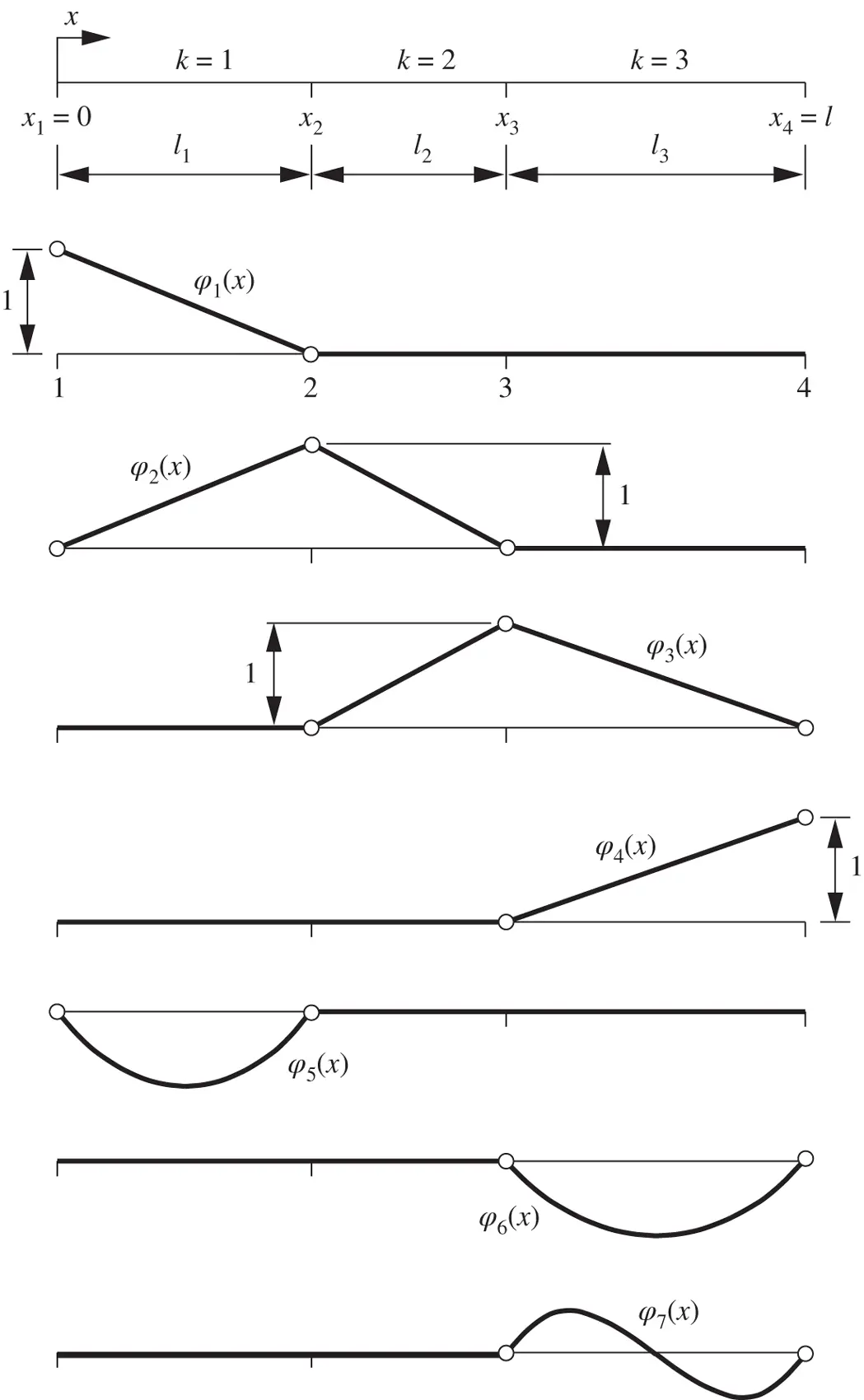
Figure 1.5 Typical finite element basis functions in one dimension.
Table 1.1 Local and global numbering in Example 1.6.
| Element number | |||||||||
|---|---|---|---|---|---|---|---|---|---|
| Numbering | 1 | 2 | 3 | ||||||
| local | 1 | 2 | 3 | 1 | 2 | 1 | 2 | 3 | 4 |
| global | 1 | 2 | 5 | 2 | 3 | 3 | 4 | 6 | 7 |
Each basis function is assigned a unique number, called a global number, and this number is associated with those element numbers and the shape function numbers from which the basis function is composed. The global and local numbers in this example are indicated in Table 1.1.
We denote 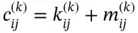 and, using equations (1.62)and (1.67), write
  in the following form:
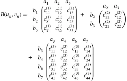
where the elements within the brackets are in the local numbering system whereas the coefficients aj and bi outside of the brackets are in the global system. The superscripts indicate the element numbers. The terms multiplied by  are summed to obtain the elements of the assembled coefficient matrix which will be denoted by
  . For example,

Assuming that the boundary conditions do not include Dirichlet conditions, the bilinear form can be written in terms of the  coefficient matrix as:
(1.76) 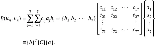
The treatment of Dirichlet conditions will be discussed separately in the next section.
The assembly of the right hand side vector from the element‐level right hand side vectors is analogous to the procedure just described. Referring to eq. (1.73)we write  in the following form:
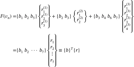
where  ,
, 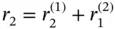 ,
, 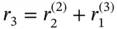 , etc.
1.3.6 Condensation
Each element has  internal basis functions. Those elements of the coefficient matrix which are associated with the internal basis functions can be eliminated at the element level. This process is called condensation.
Let us partition the coefficient matrix and right hand side vector of a finite element with  such that
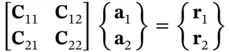
where the  and
and  . The coefficient matrix is symmetric therefore
  . Using
Интервал:
Закладка:
Похожие книги на «Finite Element Analysis»
Представляем Вашему вниманию похожие книги на «Finite Element Analysis» списком для выбора. Мы отобрали схожую по названию и смыслу литературу в надежде предоставить читателям больше вариантов отыскать новые, интересные, ещё непрочитанные произведения.


Обсуждение, отзывы о книге «Finite Element Analysis» и просто собственные мнения читателей. Оставьте ваши комментарии, напишите, что Вы думаете о произведении, его смысле или главных героях. Укажите что конкретно понравилось, а что нет, и почему Вы так считаете.