Barna Szabó - Finite Element Analysis
Здесь есть возможность читать онлайн «Barna Szabó - Finite Element Analysis» — ознакомительный отрывок электронной книги совершенно бесплатно, а после прочтения отрывка купить полную версию. В некоторых случаях можно слушать аудио, скачать через торрент в формате fb2 и присутствует краткое содержание. Жанр: unrecognised, на английском языке. Описание произведения, (предисловие) а так же отзывы посетителей доступны на портале библиотеки ЛибКат.
- Название:Finite Element Analysis
- Автор:
- Жанр:
- Год:неизвестен
- ISBN:нет данных
- Рейтинг книги:5 / 5. Голосов: 1
-
Избранное:Добавить в избранное
- Отзывы:
-
Ваша оценка:
Finite Element Analysis: краткое содержание, описание и аннотация
Предлагаем к чтению аннотацию, описание, краткое содержание или предисловие (зависит от того, что написал сам автор книги «Finite Element Analysis»). Если вы не нашли необходимую информацию о книге — напишите в комментариях, мы постараемся отыскать её.
Finite Element Analysis — читать онлайн ознакомительный отрывок
Ниже представлен текст книги, разбитый по страницам. Система сохранения места последней прочитанной страницы, позволяет с удобством читать онлайн бесплатно книгу «Finite Element Analysis», без необходимости каждый раз заново искать на чём Вы остановились. Поставьте закладку, и сможете в любой момент перейти на страницу, на которой закончили чтение.
Интервал:
Закладка:
Using five elements of equal length on the interval  and
and  assigned to each element, find the finite element solution for this problem.
Referring to equations (1.66)and (1.70), the element‐level coefficient matrix for each element is
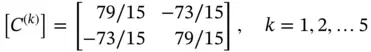
where we used  ,
,  ,
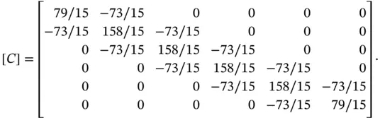
,  . The assembled unconstrained coefficient matrix is:
Upon enforcement of the Dirichlet conditions the system of equations is
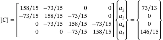
alternatively:
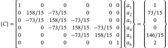
where the first and sixth equations are placeholders for the boundary conditions  ,
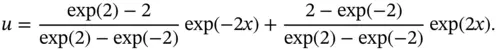
,  . The solution is:

Exercise 1.14Solve the problem in Example 1.7with the boundary conditions  ,
,  .
.
Exercise 1.15Solve the problem in Example 1.7with the boundary conditions  ,
,  .
.
1.4 Post‐solution operations
Following assembly of the coefficient matrix and enforcement of the essential boundary conditions (when applicable) the resulting system of simultaneous equations is solved by one of several methods designed to exploit the symmetry and sparsity of the coefficient matrix. The solvers are classified into two broad categories; direct and iterative solvers. Optimal choice of a solver in a particular application is based on consideration of the size of the problem and the available computational resources.
At the end of the solution process the finite element solution is available in the form
(1.81) 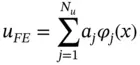
where the indices reference the global numbering and Nu is the number of degrees of freedom plus the number of Dirichlet conditions.
The basis functions are decomposed into their constituent shape functions and the element‐level solution records are created in the local numbering convention. Therefore the finite element solution on the k th element is available in the following form:
(1.82) 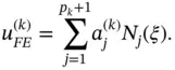
1.4.1 Computation of the quantities of interest
The computation of typical engineering quantities of interest (QoI) by direct and indirect methods is outlined in this section.
Computation of uFE ( x 0)
Direct computation of  in the point
  involves a search to identify the element Ik in which point x 0lies and, using the inverse of the mapping function defined by eq. (1.60), the standard coordinate
  corresponding to x 0is determined:
(1.83) 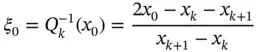
and  is computed from
(1.84) 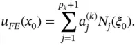
Direct computation of 
Direct computation of  in the point x 0involves the computation of the corresponding standard coordinate
  using eq. (1.83)and evaluating the following expression:
(1.85) 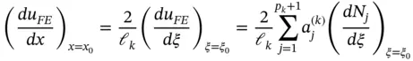
where  . The computation of the higher derivatives is analogous.
Remark 1.8When plotting quantities of interest such as the functions  and
and  , the data for the plotting routine are generated by subdividing the standard element into n intervals of equal length, n being the desired resolution. The QoIs corresponding to the grid‐points are evaluated. This process does not involve inverse mapping. In node points information is provided from the two elements that share that node. If the computed QoI is discontinuous then the discontinuity will be visible at the nodes unless the plotting algorithm automatically averages the QoIs.
Интервал:
Закладка:
Похожие книги на «Finite Element Analysis»
Представляем Вашему вниманию похожие книги на «Finite Element Analysis» списком для выбора. Мы отобрали схожую по названию и смыслу литературу в надежде предоставить читателям больше вариантов отыскать новые, интересные, ещё непрочитанные произведения.


Обсуждение, отзывы о книге «Finite Element Analysis» и просто собственные мнения читателей. Оставьте ваши комментарии, напишите, что Вы думаете о произведении, его смысле или главных героях. Укажите что конкретно понравилось, а что нет, и почему Вы так считаете.