Simon Haykin - Nonlinear Filters
Здесь есть возможность читать онлайн «Simon Haykin - Nonlinear Filters» — ознакомительный отрывок электронной книги совершенно бесплатно, а после прочтения отрывка купить полную версию. В некоторых случаях можно слушать аудио, скачать через торрент в формате fb2 и присутствует краткое содержание. Жанр: unrecognised, на английском языке. Описание произведения, (предисловие) а так же отзывы посетителей доступны на портале библиотеки ЛибКат.
- Название:Nonlinear Filters
- Автор:
- Жанр:
- Год:неизвестен
- ISBN:нет данных
- Рейтинг книги:5 / 5. Голосов: 1
-
Избранное:Добавить в избранное
- Отзывы:
-
Ваша оценка:
Nonlinear Filters: краткое содержание, описание и аннотация
Предлагаем к чтению аннотацию, описание, краткое содержание или предисловие (зависит от того, что написал сам автор книги «Nonlinear Filters»). Если вы не нашли необходимую информацию о книге — напишите в комментариях, мы постараемся отыскать её.
Discover the utility of using deep learning and (deep) reinforcement learning in deriving filtering algorithms with this insightful and powerful new resource Nonlinear Filters: Theory and Applications
Nonlinear Filters
Nonlinear Filters: Theory and Applications
Nonlinear Filters — читать онлайн ознакомительный отрывок
Ниже представлен текст книги, разбитый по страницам. Система сохранения места последней прочитанной страницы, позволяет с удобством читать онлайн бесплатно книгу «Nonlinear Filters», без необходимости каждый раз заново искать на чём Вы остановились. Поставьте закладку, и сможете в любой момент перейти на страницу, на которой закончили чтение.
Интервал:
Закладка:
From its structure, it is obvious that the observability Gramian matrix is symmetric and nonnegative. If we apply a transformation,  , to the state vector,
  , such that
  , the output energy:
(2.47) 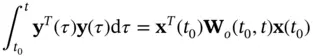
can be rewritten as:
(2.48) 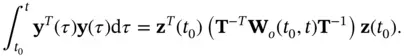
If the transformation  is chosen in a way that the transformed observability Gramian matrix,
 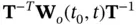 , is diagonal, then, its diagonal elements can be viewed as the contribution of different state variables in the initial state vector
  to the energy of the output. The continuous‐time LTV system of ( 2.36) and ( 2.37) is observable, if and only if the observability Gramian matrix
  is nonsingular [9, 14].
2.5.2 Discrete‐Time LTV Systems
The state‐space model of a discrete‐time LTV system is represented by the following algebraic and difference equations:
(2.49) 
(2.50) 
Before proceeding with a discussion on the observability condition, we need to define the discrete‐time state‐transition matrix ,  , as the solution of the following difference equation:
(2.51) 
with the initial condition:
(2.52) 
The reason that  is called the state‐transition matrix is that it describes the dynamic behavior of the following autonomous system (a system with no input):
(2.53) 
with  being obtained from
(2.54) 
Following a discussion on energy of the system output similar to the continuous‐time case, we reach the following definition for the discrete‐time observability Gramian matrix:
(2.55) 
As before, the system ( 2.49) and ( 2.50) is observable, if and only if the observability Gramian matrix  is full‐rank (nonsingular) [9].
2.5.3 Discretization of LTV Systems
This section generalizes the method presented before for discretization of continuous‐time LTI systems and describes how the continuous‐time LTV system ( 2.36) and ( 2.37) can be discretized. Solving the differential equation in ( 2.36), we obtain:
(2.56) 
where  is the state‐transition matrix as described in ( 2.40) and ( 2.41). Using zero‐order‐hold sampling results in a piecewise‐constant input
  , which remains constant at
  over the time interval
  . Setting
  and
and  , from ( 2.56), we will have:
(2.57) 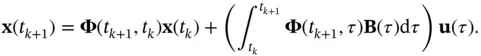
Therefore, dynamics of the discrete‐time equivalent of the continuous‐time system in ( 2.36) and ( 2.37) will be governed by the following state‐space model [19]:
(2.58) 
(2.59) 
where
(2.60) 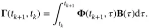
2.6 Observability of Nonlinear Systems
As mentioned before, observability is a global property for linear systems. However, for nonlinear systems, a weaker form of observability is defined, in which an initial state must be distinguishable only from its neighboring points. Two states  and
and  are indistinguishable , if their corresponding outputs are equal:
  for
for  , where
  is finite. If the set of states in the neighborhood of a particular initial state
  that are indistinguishable from it includes only
  , then, the nonlinear system is said to be weakly observable at that initial state. A nonlinear system is called to be weakly observable if it is weakly observable at all
  . If the state and the output trajectories of a weakly observable nonlinear system remain close to the corresponding initial conditions, then the system that satisfies this additional constraint is called locally weakly observable [13, 20].
Интервал:
Закладка:
Похожие книги на «Nonlinear Filters»
Представляем Вашему вниманию похожие книги на «Nonlinear Filters» списком для выбора. Мы отобрали схожую по названию и смыслу литературу в надежде предоставить читателям больше вариантов отыскать новые, интересные, ещё непрочитанные произведения.


Обсуждение, отзывы о книге «Nonlinear Filters» и просто собственные мнения читателей. Оставьте ваши комментарии, напишите, что Вы думаете о произведении, его смысле или главных героях. Укажите что конкретно понравилось, а что нет, и почему Вы так считаете.