Simon Haykin - Nonlinear Filters
Здесь есть возможность читать онлайн «Simon Haykin - Nonlinear Filters» — ознакомительный отрывок электронной книги совершенно бесплатно, а после прочтения отрывка купить полную версию. В некоторых случаях можно слушать аудио, скачать через торрент в формате fb2 и присутствует краткое содержание. Жанр: unrecognised, на английском языке. Описание произведения, (предисловие) а так же отзывы посетителей доступны на портале библиотеки ЛибКат.
- Название:Nonlinear Filters
- Автор:
- Жанр:
- Год:неизвестен
- ISBN:нет данных
- Рейтинг книги:5 / 5. Голосов: 1
-
Избранное:Добавить в избранное
- Отзывы:
-
Ваша оценка:
Nonlinear Filters: краткое содержание, описание и аннотация
Предлагаем к чтению аннотацию, описание, краткое содержание или предисловие (зависит от того, что написал сам автор книги «Nonlinear Filters»). Если вы не нашли необходимую информацию о книге — напишите в комментариях, мы постараемся отыскать её.
Discover the utility of using deep learning and (deep) reinforcement learning in deriving filtering algorithms with this insightful and powerful new resource Nonlinear Filters: Theory and Applications
Nonlinear Filters
Nonlinear Filters: Theory and Applications
Nonlinear Filters — читать онлайн ознакомительный отрывок
Ниже представлен текст книги, разбитый по страницам. Система сохранения места последней прочитанной страницы, позволяет с удобством читать онлайн бесплатно книгу «Nonlinear Filters», без необходимости каждый раз заново искать на чём Вы остановились. Поставьте закладку, и сможете в любой момент перейти на страницу, на которой закончили чтение.
Интервал:
Закладка:
Definition 2.1 (State observability) A dynamic system is state observable if for any time , the initial state can be uniquely determined from the time history of the input and the output for ; otherwise, the system is unobservable.
Unlike linear systems, there is not a universal definition for observability of nonlinear systems. Hence, different definitions have been proposed in the literature, which take two questions into consideration:
How to check the observability of a nonlinear system?
How to design an observer for such a system?
While for linear systems, observability is a global property, for nonlinear systems, observability is usually studied locally [9].
Definition 2.2 (State detectability) If all unstable modes of a system are observable, then the system is state detectable.
A system with undetectable modes is said to have hidden unstable modes [16, 17]. Sections provide observability tests for different classes of systems, whether they be linear or nonlinear, continuous‐time or discrete‐time.
2.4 Observability of Linear Time‐Invariant Systems
If the system matrices in the state‐space model of a linear system are constant, then, the model represents a linear time‐invariant (LTI) system.
2.4.1 Continuous‐Time LTI Systems
The state‐space model of a continuous‐time LTI system is represented by the following algebraic and differential equations:
(2.3)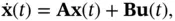
(2.4) 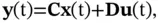
where  ,
,  , and
, and  are the state, the input, and the output vectors, respectively, and
  ,
,  ,
,  , and
, and  are the system matrices. Here, we need to find out when an initial state vector
  can be uniquely reconstructed from nonzero initial system output vector and its successive derivatives. We start by writing the system output vector and its successive derivatives based on the state vector as well as the input vector and its successive derivatives as follows:
(2.5) 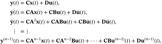
where the superscript in the parentheses denotes the order of the derivative. The aforementioned equations can be rewritten in the following compact form:
(2.6) 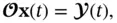
where
(2.7) 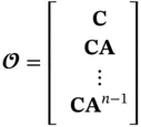
and
(2.8) 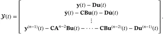
Initially we have
(2.9) 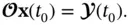
The continuous‐time system is observable, if and only if the observability matrix  is nonsingular (it is full rank), therefore the initial state can be found as:
(2.10) 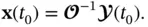
The observable subspace of the linear system, denoted by  , is composed of the basis vectors of the range of
  , and the unobservable subspace of the linear system, denoted by
  , is composed of the basis vectors of the null space of
  . These two subspaces can be combined to form the following nonsingular transformation matrix:
(2.11) 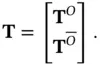
If we apply the aforementioned transformation to the state vector  such that:
(2.12) 
the transformed state vector  will be partitioned to observable modes,
  , and unobservable modes,
  :
:
(2.13) 
Then, the state‐space model of ( 2.3) and ( 2.4) can be rewritten based on the transformed state vector,  , as follows:
(2.14) 
(2.15) 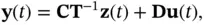
or equivalently as:
(2.16) 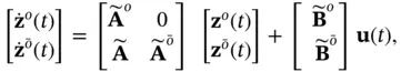
Интервал:
Закладка:
Похожие книги на «Nonlinear Filters»
Представляем Вашему вниманию похожие книги на «Nonlinear Filters» списком для выбора. Мы отобрали схожую по названию и смыслу литературу в надежде предоставить читателям больше вариантов отыскать новые, интересные, ещё непрочитанные произведения.


Обсуждение, отзывы о книге «Nonlinear Filters» и просто собственные мнения читателей. Оставьте ваши комментарии, напишите, что Вы думаете о произведении, его смысле или главных героях. Укажите что конкретно понравилось, а что нет, и почему Вы так считаете.