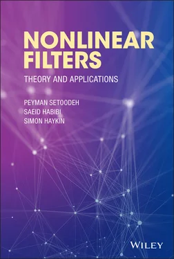
Simon Haykin - Nonlinear Filters

Chapter 10presents the expectation maximization algorithm and its variants, which are used for joint state and parameter estimation.

Chapter 11presents the reinforcement learning‐based filter, which is built on viewing variational inference and reinforcement learning as instances of a generic expectation maximization problem.

The last chapter is dedicated to nonparametric Bayesian models:

Chapter 12covers measure‐theoretic probability concepts as well as the notions of exchangeability, posterior computability, and algorithmic sufficiency. Furthermore, it provides guidelines for constructing nonparametric Bayesian models from finite parametric Bayesian models.

In each chapter, selected applications of the presented filtering algorithms are reviewed, which cover a wide range of problems. Moreover, the last section of each chapter usually refers to a few topics for further study.

In many branches of science and engineering, it is common to deal with sequential data, which is generated by dynamic systems. In different applications, it is often desirable to predict future observations based on the collected data up to a certain time instant. Since the future is always uncertain, it is preferred to have a measure that shows our confidence about the predictions. A probability distribution over possible future outcomes can provide this information [8]. A great deal of what we know about a system cannot be presented in terms of quantities that can be directly measured. In such cases, we try to build a model for the system that helps to explain the cause behind what we observe via the measurement process. This leads to the notions of state and state‐space model of a dynamic system. Chapters 3– 7and 9– 11are dedicated to different methods for reconstructing (estimating) the state of dynamic systems from inputs and measurements. Each estimation algorithm has its own advantages and limitations that should be taken into account, when we want to choose an estimator for a specific application. However, before trying to choose a proper estimation algorithm among different candidates, we need to know if for a given model of the dynamic system under study, it is possible to estimate the state of the system from inputs and measurements [9]. This critical question leads to the concept of observability , which is the focus of this chapter.

The behavioral approach for studying dynamic systems is based on an abstract model of the system of interest, which determines the relationship between its input and output. In this abstract model, the input of the system, denoted by , represents the effect of the external events on the system, and its output, denoted by , represents any change it causes to the surrounding environment. The output can be directly measured [10]. State of the system, denoted by , is defined as the minimum amount of information required at each time instant to uniquely determine the future behavior of the system provided that we know inputs to the system as well as the system's parameters. Parameter values reflect the underlying physical characteristics based on which the model of the system was built [9]. State variables may not be directly accessible for measurement; hence, the reason for calling them hidden or latent variables. Regarding the abstract nature of the state variables, they may not even represent physical quantities. However, these variables help us to improve a model's ability to capture the causal structure of the system under study [11].

A state‐space model includes the corresponding mappings from input to state and from state to output. This model also describes evolution of the system's state over time [12]. In other words, any state‐space model has three constituents [8]:

A prior, , which is associated with the initial state .

A state‐transition function, .

An observation function, .

For controlled systems, the state‐transition function depends on control inputs as well. To be able to model active perception (sensing), the observation function must be allowed to depend on inputs too.

The state‐space representation is based on the assumption that the model is a first‐order Markov process, which means that value of the state vector at cycle depends only on its value at cycle , but not on its values in previous cycles. In other words, the state vector at cycle contains all the information about the system from the initial cycle till cycle . In a sense, the concept of state inherently represents the memory of the system [13]. The first‐order Markov‐model assumption can be shown mathematically as follows:

(2.1)

It should be noted that if a model is not a first‐order Markov process, it would be possible to build a corresponding first‐order Markov model based on an augmented state vector, which includes the state vector at current cycle as well as the state vectors in previous cycles. The order of the Markov process determines that the state vectors from how many previous cycles must be included in the augmented state vector. For instance, if the system is an th‐order Markov process with state vector , the corresponding first‐order Markov model is built based on the augmented state vector:

(2.2)

Moreover, if model parameters are time‐varying, they can be treated as random variables by including them in the augmented state vector as well.

Observability and controllability are two basic properties of dynamic systems. These two concepts were first introduced by Kalman in 1960 for analyzing control systems based on linear state‐space models [1]. While observability is concerned with how the state vector influences the output vector, controllability is concerned with how the input vector influences the state vector. If a state has no effect on the output, it is unobservable ; otherwise, it is observable . To be more precise, starting from an unobservable initial state , system's output will be , in the absence of an input, [14]. Another interpretation would be that unobservable systems allow for the existence of indistinguishable states, which means that if an input is applied to the system at any one of the indistinguishable states, then the output will be the same. On the contrary, observability implies that an observer would be able to distinguish between different initial states based on inputs and measurements. In other words, an observer would be able to uniquely determine observable initial states from inputs and measurements [13, 15]. In a general case, the state vector may be divided into two parts including observable and unobservable states.