Simon Haykin - Nonlinear Filters

A rearrangement of the tuples may change the shape of the PDF curve significantly, but it does not affect the value of the summation in (2.95) or integration in (2.96), because the summation and integration can be calculated in any order. Since is not affected by local changes in the PDF curve, it can be considered as a global measure of the behavior of the corresponding PDF.

On the other hand, such a rearrangement of points changes the slope, and therefore gradient of the PDF curve, which, in turn, changes the Fisher information significantly. Hence, the Fisher information is sensitive to local rearrangement of points and can be considered as a local measure of the behavior of the corresponding PDF.

Both entropy (as a global measure of smoothness in the PDF) and Fisher information (as a local measure of smoothness in the PDF) can be used in a variational principle to infer about the PDF that describes the phenomenon under consideration. However, the local measure may be preferred in general [27]. This leads to another performance metric, which is discussed in Section 4.5.

To assess the performance of an estimator, a lower bound is always desirable. Such a bound is a measure of performance limitation that determines whether or not the design criterion is realistic and implementable. The Cramér–Rao lower bound (CRLB) is a lower bound that represents the lowest possible mean‐square error in the estimation of deterministic parameters for all unbiased estimators. It can be computed as the inverse of the Fisher information matrix. For random variables, a similar version of the CRLB, namely, the posterior Cramér–Rao lower bound (PCRLB) was derived in [52] as:

(4.19)

where denotes the inverse of Fisher information matrix at time instant . This bound is also referred to as the Bayesian CRLB [53, 54]. To compute it in an online manner, an iterative version of the PCRLB for nonlinear filtering using state‐space models was proposed in [55], where the posterior information matrix of the hidden state vector is decomposed for each discrete‐time instant by virtue of the factorization of the joint PDF of the state variables. In this way, an iterative structure is obtained for evolution of the information matrix. For a nonlinear system with the following state‐space model with zero‐mean additive Gaussian noise:

(4.20)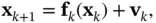

(4.21)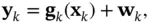

the sequence of posterior information matrices, , for estimating state vectors, , can be computed as [55]:

(4.22)

where

(4.23)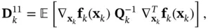

(4.24)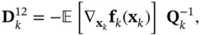

(4.25)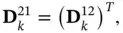

(4.26)

where and are the process and measurement noise covariance matrices, respectively.

The general formulation of the optimal nonlinear Bayesian filtering leads to a computationally intractable problem; hence, the Bayesian solution is a conceptual solution. Settling for computationally tractable suboptimal solutions through deploying different approximation methods has led to a wide range of classic as well as machine learning‐based filtering algorithms. Such algorithms have their own advantages, restrictions, and domains of applicability. To assess and compare such filtering algorithms, several performance metrics can be used including entropy, Fisher information, and PCRLB. Furthermore, the Fisher information matrix is used to define the natural gradient , which is helpful in machine learning.

Текст предоставлен ООО «ЛитРес».

Прочитайте эту книгу целиком, купив полную легальную версию на ЛитРес.

Безопасно оплатить книгу можно банковской картой Visa, MasterCard, Maestro, со счета мобильного телефона, с платежного терминала, в салоне МТС или Связной, через PayPal, WebMoney, Яндекс.Деньги, QIWI Кошелек, бонусными картами или другим удобным Вам способом.