Simon Haykin - Nonlinear Filters

(3.51)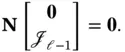

To choose , note that:

(3.52)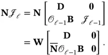

From Theorem 3.1, the first columns of must be linearly independent of each other and of the other columns. Now, is chosen such that:

(3.53)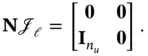

Regarding ( 3.45), can be expressed as:

(3.54)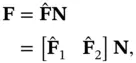

where has columns. Then, equation ( 3.45) leads to:

(3.55)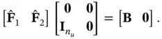

Hence, and is a free matrix. According to ( 3.46), we have:

(3.56)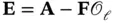

(3.57)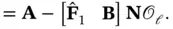

Defining , where has rows, we obtain:

(3.58)

Since is required to be a stable matrix, the pair must be detectable [35].

From ( 3.35) and ( 3.36), we have:

(3.59)

Assuming that has full column rank, there exists a matrix such that:

(3.60)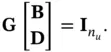

Left‐multiplying both sides of the equation ( 3.59) by , and then using ( 3.60), the input vector can be estimated based on the state‐vector estimate as:

(3.61)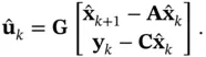

Regarding ( 3.42), this estimate asymptotically approaches the true value of the input [35].

Observers are dynamic processes, which are used to estimate the states or the unknown inputs of linear as well as nonlinear dynamic systems. This chapter covered the Luenberger observer, the extended Luenberger‐type observer, the sliding‐mode observer, and the UIO. In addition to the mentioned observers, high‐gain observers have been proposed in the literature to handle uncertainty. Although the deployed high gains in high‐gain observers allow for fast convergence and performance recovery, they amplify the effect of measurement noise [40]. Hence, there is a trade‐off between fast state reconstruction under uncertainty and measurement noise attenuation. Due to this trade‐off, in the transient and steady‐state periods, relatively high and low gains are used, respectively. However, stochastic approximation allows for an implementation of the high‐gain observer, which is able to cope with measurement noise [41]. Alternatively, the bounding observer or interval observer provides two simultaneous state estimations, which play the role of an upper bound and a lower bound on the true value of the state. The true value of the state is guaranteed to remain within these two bounds [42].

Immanuel Kant proposed the two concepts of the noumenal world and the phenomenal world. While the former is the world of things as they are, which is independent of our modes of perception and thought, the latter is the world of things as they appear to us, which depends on how we perceive things. According to Kant, everything about the noumenal world is transcendental that means it exists but is not prone to concept formation by us [43].

Following this line of thinking, statistics will aim at interpretation rather than explanation. In this framework, statistical inference is built on probabilistic modeling of the observed phenomenon. A probabilistic model must include the available information about the phenomenon of interest as well as the uncertainty associated with this information. The purpose of statistical inference is to solve an inverse problem aimed at retrieving the causes, which are presented by states and/or parameters of the developed probabilistic model, from the effects, which are summarized in the observations. On the other hand, probabilistic modeling describes the behavior of the system and allows us to predict what will be observed in the future conditional on states and/or parameters [44].