Simon Haykin - Nonlinear Filters

Bayesian paradigm provides a mathematical framework in which degrees of belief are quantified by probabilities. It is the method of choice for dealing with uncertainty in measurements. Using the Bayesian approach, probability of an event of interest (state) can be calculated based on the probability of other events (observations or measurements) that are logically connected to and therefore, stochastically dependent on the event of interest. Moreover, the Bayesian method allows us to iteratively update probability of the state when new measurements become available [45]. This chapter reviews the Bayesian paradigm and presents the formulation of the optimal nonlinear filtering problem.

Bayes' theorem describes the inversion of probabilities. Let us consider two events and . Provided that , we have the following relationship between the conditional probabilities and :

(4.1)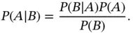

Considering two random variables and with conditional distribution and marginal distribution ), the continuous version of Bayes' rule is as follows:

(4.2)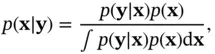

where is the prior distribution, is the posterior distribution, and is the likelihood function, which is also denoted by . This formula captures the essence of Bayesian statistical modeling, where denotes observations, and represents states or parameters. In order to build a Bayesian model, we need a parametric statistical model described by the likelihood function . Furthermore, we need to incorporate our knowledge about the system under study and the uncertainty about this information, which is represented by the prior distribution [44].

The following discrete‐time stochastic state‐space model describes the behavior of a discrete‐time nonlinear system:

(4.3)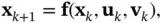

(4.4)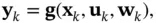

where , , and denote the state, the input, and the output vectors, respectively. Compared with the deterministic nonlinear discrete‐time model in (2.78) and (2.79), two additional variables are included in the above stochastic model, which are the process noise, , and the measurement noise, . These two random variables take account of model inaccuracies and other sources of uncertainty. The more accurate the model is, the smaller the contribution of noise terms will be. These two noise sequences are assumed to be white, independent of each other, and independent from the initial state. The probabilistic model of the state evolution in ( 4.3) is assumed to be a first‐order Markov process, and therefore, can be rewritten as the following state‐transition probability density function (PDF) [46]:

(4.5)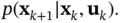

Similarly, the measurement model in ( 4.4) can be represented by the following PDF:

(4.6)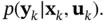

The input sequence and the available measurement sequence at time instant are denoted by and , respectively. These two sequences form the available information at time , hence the union of these two sets is called the information set , [47].