Simon Haykin - Nonlinear Filters

A filter uses the inputs and available observations up to time instant , to estimate the state at , . In other words, a filter tries to solve an inverse problem to infer the states (cause) from the observations (effect). Due to uncertainties, different values of the state could have led to the obtained measurement sequence, . The Bayesian framework allows us to associate a degree of belief to these possibly valid values of state. The main idea here is to start from an initial density for the state vector, , and recursively calculate the posterior PDF, based on the measurements. This can be done by a filtering algorithm that includes two‐stages of prediction and update [46].

In the prediction stage, the Chapman–Kolmogorov equation can be used to calculate the prediction density, , from , which is provided by the update stage of the previous iteration. Using ( 4.5), the prediction density can be computed as [46, 47]:

(4.7)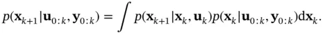

When a new measurement is obtained, the prediction stage is followed by the update stage, where the above prediction density will play the role of the prior. Bayes' rule is used to compute the posterior density of the state as [46, 47]:

(4.8)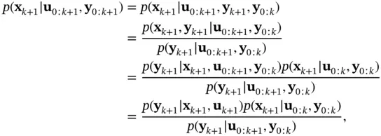

where the normalization constant in the denominator is obtained as:

(4.9)

The recursive propagation of the state posterior density according to equations ( 4.7) and ( 4.8) provides the basis of the Bayesian solution . Having the posterior, , the optimal state estimate can be obtained based on a specific criterion. Depending on the chosen criterion, different estimators are obtained [46–48]:

Minimum mean‐square error (MMSE) estimator(4.10) This is equivalent to minimizing the trace (sum of the diagonal elements) of the estimation‐error covariance matrix. The MMSE estimate is the conditional mean of :(4.11) where the expectation is taken with respect to the posterior, .

Risk‐sensitive (RS) estimator(4.12) Compared to the MMSE estimator, the RS estimator is less sensitive to uncertainties. In other words, it is a more robust estimator [49].

Maximum a posteriori (MAP) estimator(4.13)

Minimax estimator(4.14) The minimax estimate is the medium of the posterior, . The minimax technique is used to achieve optimal performance under the worst‐case condition [50].

The most probable (MP) estimator(4.15) MP estimate is the mode of the posterior, . For a uniform prior, this estimate will be identical to the maximum likelihood (ML) estimate.(4.16)

In general, there may not exist simple analytic forms for the corresponding PDFs. Without an analytic form, the PDF for a single variable will be equivalent to an infinite‐dimensional vector that must be stored for performing the required computations. In such cases, obtaining the Bayesian solution will be computationally intractable. In other words, the Bayesian solution except for special cases, is a conceptual solution, and generally speaking, it cannot be determined analytically. In many practical situations, we will have to use some sort of approximation, and therefore, settle for a suboptimal Bayesian solution [46]. Different approximation methods lead to different filtering algorithms.

The relevant portion of the data obtained by measurement can be interpreted as information. In this line of thinking, a summary of the amount of information with regard to the variables of interest is provided by the Fisher information matrix [51]. To be more specific, Fisher information plays two basic roles:

1 It is a measure of the ability to estimate a quantity of interest.

2 It is a measure of the state of disorder in a system or phenomenon of interest.

The first role implies that the Fisher information matrix has a close connection to the estimation‐error covariance matrix and can be used to calculate the confidence region of estimates. The second role implies that the Fisher information has a close connection to Shannon's entropy.

Let us consider the PDF , which is parameterized by the set of parameters . The Fisher information matrix is defined as:

(4.17)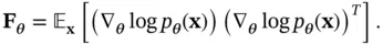

This definition is based on the outer product of the gradient of with itself, where the gradient is a column vector denoted by . There is an equivalent definition based on the second derivative of as:

(4.18)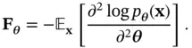

From the definition of , it is obvious that Fisher information is a function of the corresponding PDF. A relatively broad and flat PDF, which is associated with lack of predictability and high entropy, has small gradient contents and, in effect therefore, low Fisher information. On the other hand, if the PDF is relatively narrow and has sharp slopes around a specific value of , which is associated with bias toward that particular value of and low entropy, it has large gradient contents and therefore high Fisher information. In summary, there is a duality between Shannon's entropy and Fisher information. However, a closer look at their mathematical definitions reveals an important difference [27]: