Simon Haykin - Nonlinear Filters
Здесь есть возможность читать онлайн «Simon Haykin - Nonlinear Filters» — ознакомительный отрывок электронной книги совершенно бесплатно, а после прочтения отрывка купить полную версию. В некоторых случаях можно слушать аудио, скачать через торрент в формате fb2 и присутствует краткое содержание. Жанр: unrecognised, на английском языке. Описание произведения, (предисловие) а так же отзывы посетителей доступны на портале библиотеки ЛибКат.
- Название:Nonlinear Filters
- Автор:
- Жанр:
- Год:неизвестен
- ISBN:нет данных
- Рейтинг книги:5 / 5. Голосов: 1
-
Избранное:Добавить в избранное
- Отзывы:
-
Ваша оценка:
Nonlinear Filters: краткое содержание, описание и аннотация
Предлагаем к чтению аннотацию, описание, краткое содержание или предисловие (зависит от того, что написал сам автор книги «Nonlinear Filters»). Если вы не нашли необходимую информацию о книге — напишите в комментариях, мы постараемся отыскать её.
Discover the utility of using deep learning and (deep) reinforcement learning in deriving filtering algorithms with this insightful and powerful new resource Nonlinear Filters: Theory and Applications
Nonlinear Filters
Nonlinear Filters: Theory and Applications
Nonlinear Filters — читать онлайн ознакомительный отрывок
Ниже представлен текст книги, разбитый по страницам. Система сохранения места последней прочитанной страницы, позволяет с удобством читать онлайн бесплатно книгу «Nonlinear Filters», без необходимости каждый раз заново искать на чём Вы остановились. Поставьте закладку, и сможете в любой момент перейти на страницу, на которой закончили чтение.
Интервал:
Закладка:
the transformed state vector  will be partitioned to observable modes,
  , and unobservable modes,
  :
:
(2.27) 
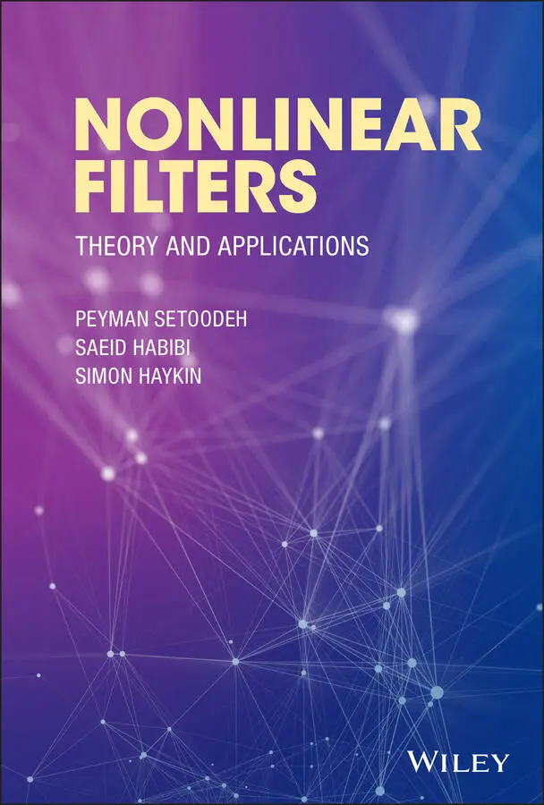
Then, the state‐space model of ( 2.18) and ( 2.19) can be rewritten based on the transformed state vector,  , as follows:
(2.28) 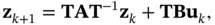
(2.29) 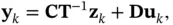
or equivalently as:
(2.30) 
(2.31) 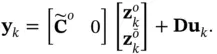
Any pair of equations ( 2.28) and ( 2.29) or ( 2.30) and ( 2.31) is called the state‐space model of the system in the observable canonical form.
2.4.3 Discretization of LTI Systems
When a continuous‐time system is connected to a computer via analog‐to‐digital and digital‐to‐analog converters at input and output, respectively, we need to find a discrete‐time equivalent of the continuous‐time system that describes the relationship between the system's input and its output at certain time instants (sampling times  for
for  ). This process is called sampling the continuous‐time system. Using zero‐order‐hold sampling, where the corresponding analog signals are kept constant over the sampling period, we will have the following discrete‐time equivalent for the continuous‐time system of ( 2.3) and ( 2.4) [18]:
(2.32) 
(2.33) 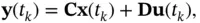
where
(2.34) 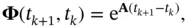
(2.35) 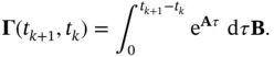
2.5 Observability of Linear Time‐Varying Systems
If the system matrices in the state‐space model of a linear system change with time, then, the model represents a linear time‐varying (LTV) system. Obviously, the observability condition would be more complicated for LTV systems compared to LTI systems.
2.5.1 Continuous‐Time LTV Systems
The state‐space model of a continuous‐time LTV system is represented by the following algebraic and differential equations:
(2.36) 
(2.37) 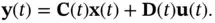
In order to determine the relative observability of different state variables, we investigate their contributions to the energy of the system output. Knowing the input, we can eliminate its contribution to the energy of the output. Therefore, without loss of generality, we can assume that the input is zero. Without an input, evolution of the state vector is governed by the following unforced differential equation:
(2.38) 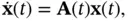
whose solution is:
(2.39) 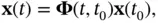
where  is called the continuous‐time state‐transition matrix , which is itself the solution of the following differential equation:
(2.40) 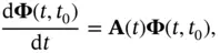
with the initial condition:
(2.41) 
Note that for an LTI system, where the matrix  is constant, the state transition matrix will be:
(2.42) 
Without an input, output of the unforced system is obtained from ( 2.37) as follows:
(2.43) 
Replacing for  from ( 2.39) in the aforementioned equation, we will have:
(2.44) 
whose energy is obtained from:
(2.45) 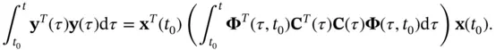
In the aforementioned equation, the matrix in the parentheses is called the continuous‐time observability Gramian matrix:
(2.46) 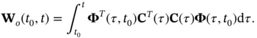
Интервал:
Закладка:
Похожие книги на «Nonlinear Filters»
Представляем Вашему вниманию похожие книги на «Nonlinear Filters» списком для выбора. Мы отобрали схожую по названию и смыслу литературу в надежде предоставить читателям больше вариантов отыскать новые, интересные, ещё непрочитанные произведения.


Обсуждение, отзывы о книге «Nonlinear Filters» и просто собственные мнения читателей. Оставьте ваши комментарии, напишите, что Вы думаете о произведении, его смысле или главных героях. Укажите что конкретно понравилось, а что нет, и почему Вы так считаете.