Simon Haykin - Nonlinear Filters

There is another difference between linear and nonlinear systems regarding observability and that is the role of inputs in nonlinear observability. While inputs do not affect the observability of a linear system, in nonlinear systems, some initial states may be distinguishable for some inputs and indistinguishable for others. This leads to the concept of uniform observability , which is the property of a class of systems, for which initial states are distinguishable for all inputs [12, 20]. Furthermore, in nonlinear systems, distinction between time‐invariant and time‐varying systems is not critical because by adding time as an extra state such as , the latter can be converted to the former [21].

The state‐space model of a continuous‐time nonlinear system is represented by the following system of nonlinear equations:

(2.61)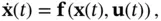

(2.62)

where 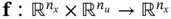is the system function, and 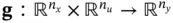is the measurement function. It is common practice to deploy a control law that uses state feedback. In such cases, the control input is itself a function of the state vector . Before proceeding, we need to recall the concept of Lie derivative from differential geometry [22, 23]. Assuming that and are smooth vector functions (they have derivatives of all orders or they can be differentiated infinitely many times), the Lie derivative of (the th element of ) with respect to is a scalar function defined as:

(2.63)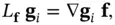

where denotes the gradient with respect to . For simplicity, arguments of the functions have not been shown. Repeated Lie derivatives are defined as:

(2.64)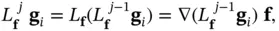

with

(2.65)

Relevance of Lie derivatives to observability of nonlinear systems becomes clear, when we consider successive derivatives of the output vector as follows:

(2.66)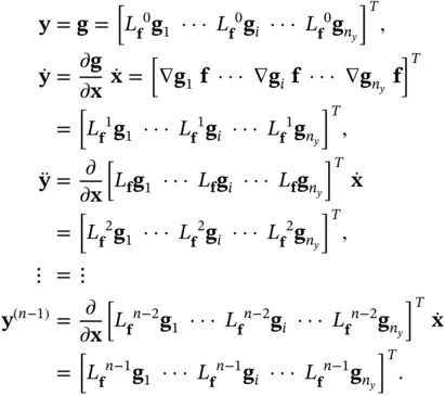

The aforementioned differential equations can be rewritten in the following compact form:

(2.67)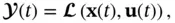

where

(2.68)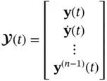

and

(2.69)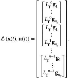

The system of nonlinear differential equations in ( 2.67) can be linearized about an initial state to develop a test for local observability of the nonlinear system ( 2.61) and ( 2.62) at this specific initial state, where the linearized test would be similar to the observability test for linear systems. Writing the Taylor series expansion of the function about and ignoring higher‐order terms, we will have:

(2.70)

Using Cartan's formula:

(2.71)

we obtain:

(2.72)

Now, we can proceed with deriving the local observability test for nonlinear systems based on the aforementioned linearized system of equations. The nonlinear system in ( 2.61) and ( 2.62) is observable at , if there exists a neighborhood of and an ‐tuple of integers called observability indices such that [9, 24]: