Simon Haykin - Nonlinear Filters
Здесь есть возможность читать онлайн «Simon Haykin - Nonlinear Filters» — ознакомительный отрывок электронной книги совершенно бесплатно, а после прочтения отрывка купить полную версию. В некоторых случаях можно слушать аудио, скачать через торрент в формате fb2 и присутствует краткое содержание. Жанр: unrecognised, на английском языке. Описание произведения, (предисловие) а так же отзывы посетителей доступны на портале библиотеки ЛибКат.
- Название:Nonlinear Filters
- Автор:
- Жанр:
- Год:неизвестен
- ISBN:нет данных
- Рейтинг книги:5 / 5. Голосов: 1
-
Избранное:Добавить в избранное
- Отзывы:
-
Ваша оценка:
Nonlinear Filters: краткое содержание, описание и аннотация
Предлагаем к чтению аннотацию, описание, краткое содержание или предисловие (зависит от того, что написал сам автор книги «Nonlinear Filters»). Если вы не нашли необходимую информацию о книге — напишите в комментариях, мы постараемся отыскать её.
Discover the utility of using deep learning and (deep) reinforcement learning in deriving filtering algorithms with this insightful and powerful new resource Nonlinear Filters: Theory and Applications
Nonlinear Filters
Nonlinear Filters: Theory and Applications
Nonlinear Filters — читать онлайн ознакомительный отрывок
Ниже представлен текст книги, разбитый по страницам. Система сохранения места последней прочитанной страницы, позволяет с удобством читать онлайн бесплатно книгу «Nonlinear Filters», без необходимости каждый раз заново искать на чём Вы остановились. Поставьте закладку, и сможете в любой момент перейти на страницу, на которой закончили чтение.
Интервал:
Закладка:
1 for .
2 The row vectors of are linearly independent.
From the row vectors  , an observability matrix can be constructed for the continuous‐time nonlinear system in ( 2.61) and ( 2.62) as follows:
(2.73) 
If  is full‐rank, then the nonlinear system in ( 2.61) and ( 2.62) is locally weakly observable. It is worth noting that the observability matrix for continuous‐time linear systems ( 2.7) is a special case of the observability matrix for continuous‐time nonlinear systems ( 2.73). In other words, if
  and
and  are linear functions, then ( 2.73) will be reduced to ( 2.7) [9, 24].
The nonlinear system in ( 2.61) and ( 2.62) can be linearized about  . Using Taylor series expansion and ignoring higher‐order terms, we will have the following linearized system:
(2.74) 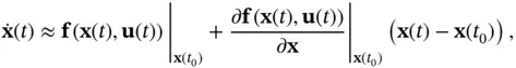
(2.75) 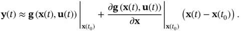
Then, the observability test for linear systems can be applied to the following linearized system matrices:
(2.76) 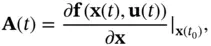
(2.77) 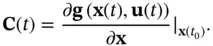
In this way, the nonlinear observability matrix in ( 2.73) can be approximated by the observability matrix, which is constructed using  and
and  in ( 2.76) and ( 2.77). Although this approach may seem simpler, observability of the linearized system may not imply the observability of the original nonlinear system [9].
2.6.2 Discrete‐Time Nonlinear Systems
The state‐space model of a discrete‐time nonlinear system is represented by the following system of nonlinear equations:
(2.78) 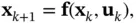
(2.79) 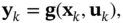
where 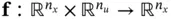 is the system function, and
 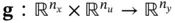 is the measurement function. Similar to the discrete‐time linear case, starting from the initial cycle, system's output vectors at successive cycles till cycle
  can be written based on the initial state
  and input vectors
  as follows:
(2.80) 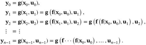
Functional powers of the system function  can be used to simplify the notation in the aforementioned equations. Functional powers are obtained by repeated composition of a function with itself:
(2.81) 
where  denotes the function‐composition operator:
 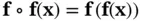 , and
, and  is the identity map. Alternatively, the difference equations in ( 2.80) can be rewritten as:
(2.82) 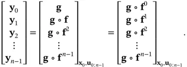
Similar to the continuous‐time case, the system of nonlinear difference equations in ( 2.82) can be linearized about the initial state  based on the Taylor series expansion to develop a linearized test for weak local observability of the nonlinear discrete‐time system ( 2.78) and ( 2.79). The nonlinear system in ( 2.78) and ( 2.79) is locally weakly observable at
  , if there exist a neighborhood of
  and an
  ‐tuple of integers
  such that [9, 25]:
1 for .
2 The following observability matrix is full rank: (2.83)
where
(2.84) 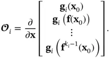
Интервал:
Закладка:
Похожие книги на «Nonlinear Filters»
Представляем Вашему вниманию похожие книги на «Nonlinear Filters» списком для выбора. Мы отобрали схожую по названию и смыслу литературу в надежде предоставить читателям больше вариантов отыскать новые, интересные, ещё непрочитанные произведения.


Обсуждение, отзывы о книге «Nonlinear Filters» и просто собственные мнения читателей. Оставьте ваши комментарии, напишите, что Вы думаете о произведении, его смысле или главных героях. Укажите что конкретно понравилось, а что нет, и почему Вы так считаете.