Daniel J. Duffy - Numerical Methods in Computational Finance
Здесь есть возможность читать онлайн «Daniel J. Duffy - Numerical Methods in Computational Finance» — ознакомительный отрывок электронной книги совершенно бесплатно, а после прочтения отрывка купить полную версию. В некоторых случаях можно слушать аудио, скачать через торрент в формате fb2 и присутствует краткое содержание. Жанр: unrecognised, на английском языке. Описание произведения, (предисловие) а так же отзывы посетителей доступны на портале библиотеки ЛибКат.

- Название:Numerical Methods in Computational Finance
- Автор:
- Жанр:
- Год:неизвестен
- ISBN:нет данных
- Рейтинг книги:4 / 5. Голосов: 1
-
Избранное:Добавить в избранное
- Отзывы:
-
Ваша оценка:
Numerical Methods in Computational Finance: краткое содержание, описание и аннотация
Предлагаем к чтению аннотацию, описание, краткое содержание или предисловие (зависит от того, что написал сам автор книги «Numerical Methods in Computational Finance»). Если вы не нашли необходимую информацию о книге — напишите в комментариях, мы постараемся отыскать её.
Part A Mathematical Foundation for One-Factor Problems
Chapters 1 to 7 introduce the mathematical and numerical analysis concepts that are needed to understand the finite difference method and its application to computational finance.
Part B Mathematical Foundation for Two-Factor Problems
Chapters 8 to 13 discuss a number of rigorous mathematical techniques relating to elliptic and parabolic partial differential equations in two space variables. In particular, we develop strategies to preprocess and modify a PDE before we approximate it by the finite difference method, thus avoiding ad-hoc and heuristic tricks.
Part C The Foundations of the Finite Difference Method (FDM)
Chapters 14 to 17 introduce the mathematical background to the finite difference method for initial boundary value problems for parabolic PDEs. It encapsulates all the background information to construct stable and accurate finite difference schemes.
Part D Advanced Finite Difference Schemes for Two-Factor Problems
Chapters 18 to 22 introduce a number of modern finite difference methods to approximate the solution of two factor partial differential equations. This is the only book we know of that discusses these methods in any detail.
Part E Test Cases in Computational Finance
Chapters 23 to 26 are concerned with applications based on previous chapters. We discuss finite difference schemes for a wide range of one-factor and two-factor problems.
This book is suitable as an entry-level introduction as well as a detailed treatment of modern methods as used by industry quants and MSc/MFE students in finance. The topics have applications to numerical analysis, science and engineering.
More on computational finance and the author’s online courses, see www.datasim.nl.
Numerical Methods in Computational Finance — читать онлайн ознакомительный отрывок
Ниже представлен текст книги, разбитый по страницам. Система сохранения места последней прочитанной страницы, позволяет с удобством читать онлайн бесплатно книгу «Numerical Methods in Computational Finance», без необходимости каждый раз заново искать на чём Вы остановились. Поставьте закладку, и сможете в любой момент перейти на страницу, на которой закончили чтение.
Интервал:
Закладка:
Some test code is:
int main() { std::cout ≪ "How many steps (need many e.g. 300000?): "; std::cin ≫ NT; CurveEuler(); CurveRichardson(); std::cout ≪ "Value at T = " ≪ U ≪ " is " ≪ std::setprecision(7) ≪ yValues[yValues.size() - 1] ≪ ", press the ANY key " ≪ std::endl; std::cout ≪ "Richardson at T = " ≪ U ≪ " is " ≪RichValues[yRichValues.size() - 1] ≪ ", press the ANY key "; // Beautiful Excel output ExcelDriver xl; xl.MakeVisible(true); xl.CreateChart(tValues, yValues, std::string("Euler for Riccati")); xl.CreateChart (tValues, yRichValues, std::string("Richardson for Riccati")); return 0; }
What is the accuracy of these schemes, and how much computer effort (size of NT and the number of function calls) is needed in order to achieve a given accuracy? To this end, we take two cases whose exact solutions have been computed using Boost C++ odeint :
Case I: , .
Case II: , .
In general, the library needs approximately 100 function evaluations to reach this level of accuracy. The results for explicit Euler and the extrapolated scheme for cases I and II for NT = 300, 500, 1000 and 5000 are:
Case I: (9.2746e-6, 1.113e-5), (1.0015e-5, 1.118e-5), (1.059e-5, 1.200e-5), (1.083e-5, 1.1206e-5).
Case II: (0.0554, 0.0559), (0.0556, 0.0559), (0.0558, 0.0559), (0.05589, 0.0559).
For a more complete discussion of Boost odeint , see Duffy (2018).
We complete our discussion of finite difference methods for (3.10). The full problem is (3.11); (3.12)is a coupled system of equations, and it can be solved in different ways. The most effective approach at this stage is to use a production third-party ODE solver in C++.
3.7 MATRIX DIFFERENTIAL EQUATIONS
We have seen what scalar and vector ODEs are. Now we consider matrix ODEs.
The Boost odeint library can be used to solve matrix ODEs, for example:
(3.25) 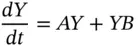
where A , B and Y are  matrices.
It can be shown that the solution of system (3.25)can be written as (see Brauer and Nohel (1969)):
(3.26) 
A special case is when:
(3.27) 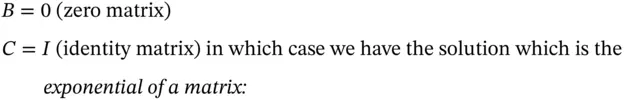
(3.28) 
The conclusion is that we can now compute the exponential of a matrix by solving a matrix ODE. We now discuss this topic using C++. To this end, we examine the system:
(3.29) 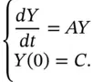
where C is a given matrix.
We model this system by the following C++ class:
namespace ublas = boost::numeric::ublas; using value_type = double; using state_type = boost::numeric::ublas::matrix; class MatrixOde { private: // dB/dt = A*B, B(0) = C; ublas::matrix A_; ublas::matrix C_; public: MatrixOde(const ublas::matrix& A, const ublas::matrix& IC) : A_(A), C_(IC) {} void operator()(const state_type &x , state_type &dxdt, double t ) const { for( std::size_t i=0 ; i < x.size1();++i ) { for( std::size_t j=0 ; j < x.size2(); ++j ) { dxdt(i, j) = 0.0; for (std::size_t k = 0; k < x.size2(); ++k) { dxdt(i, j) += A_(i,k)*x(k,j); } } } } };
There are many dubious ways to compute the exponential of a matrix, see Moler and Van Loan (2003), one of which involves the application of ODE solvers. Other methods include:
S1: Series methods (for example, truncating the infinite Taylor series representation for the exponential).
S2: Padé rational approximant. This entails approximating the exponential by a special kind of rational function.
S3: Polynomial methods using the Cayley–Hamilton method.
S4: Inverse Laplace transform.
S5: Matrix decomposition methods.
S6: Splitting methods.
3.7.1 Transition Rate Matrices and Continuous Time Markov Chains
An interesting application of matrices and matrix ODEs is to the modelling of credit rating applications (Wilmott (2006), vol. 2, pp. 665–73). To this end, we define a so-called transition matrix P , which is a table whose elements are probabilities representing migrations from one credit rating to another credit rating. For example, a company having a B rating has a probability 0.07 of getting a BB rating in a small period of time. More generally, we are interested in continuous-time transitions between states using Markov chains , and we have the following Kolmogorov forward equation :
(3.30) 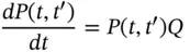
where 
 and
and  unit matrix and
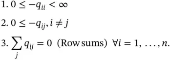
  is the transition rate matrix having the following properties:
The Kolmogorov backward equation is:
(3.31) 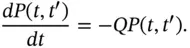
The objective is to compute the transition rate matrix Q (that is, states that are in one-to-one correspondence with the integers).
In the case of countable space, the Kolmogorov forward equation is:
(3.32) 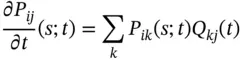
where Q ( t ) is the transition rate matrix (also known as generator matrix ), while the Kolmogorov backward equation is:
(3.33) 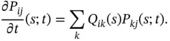
3.8 SUMMARY AND CONCLUSIONS
Интервал:
Закладка:
Похожие книги на «Numerical Methods in Computational Finance»
Представляем Вашему вниманию похожие книги на «Numerical Methods in Computational Finance» списком для выбора. Мы отобрали схожую по названию и смыслу литературу в надежде предоставить читателям больше вариантов отыскать новые, интересные, ещё непрочитанные произведения.


Обсуждение, отзывы о книге «Numerical Methods in Computational Finance» и просто собственные мнения читателей. Оставьте ваши комментарии, напишите, что Вы думаете о произведении, его смысле или главных героях. Укажите что конкретно понравилось, а что нет, и почему Вы так считаете.