Daniel J. Duffy - Numerical Methods in Computational Finance

System (3.14)is sometimes called the Lotka–Volterra equations, which are an example of a more general Kolmogorov model to model the dynamics of ecological systems with predator-prey interactions, competition, disease and mutualism (Lotka (1956)).

A logistic function (or logistic curve ) is an S-shaped sigmoid curve defined by the equation:

(3.15)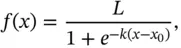

where

-value of sigmoid's midpoint

curve's maximum value

steepness of the curve.

A special case is when 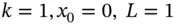, resulting in the standard logistic function defined by the equation:

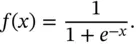
We can verify from this equation that the logistic function satisfies the non-linear initial value problem:

(3.16)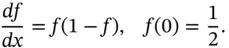

The logistic function models processes in a range of fields such as artificial neural networks (learning algorithms, where it is called an activation function ), economics, probability and statistics, to name a few.

A random process is a family of random variables defined on some probability space and indexed by the parameter t where t belongs to some index set. A random process is a function of two variables:

where T is the index set and S is the sample space . For a fixed value of t , the random process becomes a random variable, while for a fixed sample point x in S the random process is a real-valued function of t called a sample function or a realisation of the process. It is also sometimes called a path .

The index set T is called the parameter set, and the values assumed by are called the states ; finally, the set of all possible values is called the state space of the random process.

The index set T can be discrete or continuous; if T is discrete, then the process is called a discrete-parameter or discrete-time process (also known as a random sequence ). If T is continuous, then we say that the random process is called continuous-parameter or continuous-time . We can also consider the situation where the state is discrete or continuous. We then say that the random process is called discrete-state (chain) or continuous-state , respectively.

We give a short introduction to stochastic differential equations (SDEs) as they are closely related to ODEs. We discuss SDEs in more detail in Chapter 13.

We introduce the scalar random processes described by SDEs of the form:

(3.17)

where:

random process

transition (drift) coefficient

diffusion coefficient

Brownian process

given initial condition

defined in the interval [0, T ]. We assume for the moment that the process takes values on the real line. We know that this SDE can be written in the equivalent integral form:

(3.18)

This is a non-linear equation, because the unknown random process appears on both sides of the equation and it cannot be expressed in a closed form. We know that the second integral:

is a continuous process (with probability 1) provided is a bounded process. In particular, we restrict the scope to those functions for which:

Using this fact, we shall see that the solution of Equation (3.17)is bounded and continuous with probability 1.

We now discuss existence and uniqueness theorems. First, we define some conditions on the coefficients in Equation (3.17):

C1: such that .

C2: , such that

C3: and are defined and measurable with respect to their variables where .

C4: and are continuous with respect to their variables for .

Condition C2 is called a Lipschitz condition in the second variable, while condition C1 constrains the growth of the coefficients in Equation (3.17). We assume throughout that the random variable is independent of W ( t ).

Theorem 3.2Assume conditions C1, C2 and C3 hold. Then Equation (3.17)has a unique continuous solution with probability 1 for any initial condition .

Theorem 3.3Assume that conditions C1 and C4 hold. Then the Equation (3.17)has a continuous solution with probability 1 for any initial condition .

We note the difference between the two theorems: the condition C2 is what makes the solution unique. Finally, both theorems assume that is independent of the Brownian motion W ( t ).