Daniel J. Duffy - Numerical Methods in Computational Finance

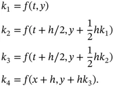
(3.22)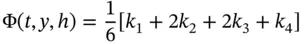

where:

Other methods are:

Second-order Ralston method :

(3.23)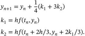

and Heun's (improved Euler) method:

(3.24)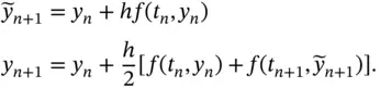

This is a predictor-corrector method that also has applications to stochastic differential equations.

In general, explicit Runge–Kutta methods are unsuitable for stiff ODEs.

We show hand-crafted code for the explicit Euler method as well as the schemes (3.22), (3.23)and (3.24). The main reason is to get hands-on experience with coding solvers for ODEs before using production solvers (for example, Python's or Boost C++ odeint libraries), especially for readers for whom numerical ODEs are new, for example readers with an economics or econometrics background. A good strategy is 1) get it working (write your own code and examples), then 2) get it right (use a library with the same examples) and then and only then get it optimised (use a library in a larger application).

The following code is for the methods:

Explicit Euler

Fourth-order Runge–Kutta (RK4)

Second-order Ralston.

Heun (improved Euler)

Predictor-corrector method.

We now present the code for a scalar IVP for these methods:

# y' = f(x,y) Explicit Euler method, scalar def Euler(f, x, y, T, N, TOL): h = (T - x) / N for n in range(1,N+1): ynP1 = y + h*f(x,y) # Go to next level x += h y = ynP1 return ynP1 # y' = f(x,y) Explicit Euler method, system def Euler2(f, x, y0, T, N, TOL): h = (T - x) / N m = len(y0) ynP1 = y0 for n in range(N): for j in range(m): ynP1[j] = y0[j] + h*f[j](x,y0) # Go to next level x += h y0 = ynP1 return ynP1 def RK4(f, x, y, T, N, TOL): # Order 4 Runge Kutta method h = (T - x) / N k1 = 0; k2 = 0; k3 = 0; k4 = 0 ynP1 = 0 # y(n+1) for n in range(N): k1 = f(x, y); k2 = f(x + h / 2, y + h*k1 / 2) k3 = f(x + h / 2, y + h*k2 / 2); k4 = f(x + h, y + h*k3); ynP1 = y + h*(k1 + 2*k2 + 2*k3 + k4)/6 # Go to next level x += h; y = ynP1 return ynP1 # https://en.wikipedia.org/wiki/Heun%27s_methoddef Heun(f, x, y, T, N, TOL): # Modified Euler method (improved polygon method), Collatz 1960 h = (T - x) / N # Variables k1 = 0; k2 = 0 for n in range(N): ynP1 = y + h*f(x+h/2, y + h*f(x,y)/2) # Go to next level x += h; y = ynP1 return ynP1 def Ralston2(f, x, y, T, N, TOL): h = (T - x) / N # Variables k1 = 0; k2=0 ynP1=0 # y(n+1) for n in range(N): k1 = h*f(x, y); k2 = h*f(x + 2*h / 3, y + 2*k1 / 3) ynP1 = y + (k1 + 3 * k2 ) / 4 # Go to next level x += h; y = ynP1 return ynP1; def PredictorCorrector(f, x, y, T, N, TOL): # PC with fixed step size h = (T - x) / N for n in range(1,N+1): yCorr2 = y + h*f(x, y) # 1. Predictor (explicit Euler) # Produce y(n+1) at level x(n+1) from level n, Inner iteration diff = 2 * TOL while (diff > TOL): yCorr = y + 0.5*h*(f(x, y) + f(x + h, yCorr2)) diff = math.fabs(yCorr - yCorr2) / math.fabs(yCorr) yCorr2 = yCorr # Stuff has converged at level n+1, now update next level x += h y = yCorr return yCorr

A sample test program is:

# TestFDMSchemes.py # # A catalogue of hand-crafted numerical methods for solving ODEs # # (C) Datasim Education BV 2021 # # Testing import math import numpy as np import FDMSchemes as fdm def func(t,y): return y*(1.0 - y) # logistic ode t = 0; y = 0.5 #initial time and value T = 4.0 #end of integration interval N = 4000 #number of divisions of [0,T] TOL = 1.0e-5 #for some method, a measure of the desired accuracy # y' = f(x,y) Explicit Euler method value = fdm.Euler(func,t,y,T,N,TOL) #scalar print(value) value = fdm.PredictorCorrector(func,t,y,T,N,TOL) #scalar print(value) value = fdm.RK4(func,t,y,T,N,TOL) #scalar print(value) y = 0.5 value = fdm.Heun(func,t,y,T,N,TOL) #scalar print(value) value = fdm.Ralston2(func,t,y,T,N,TOL) #scalar print(value)

No doubt the code can be modified to make it more “pythonic” (whatever that means) and reduce the number of lines of code (at the possible expense of readability) if that is a requirement. We have also written these algorithms in C++11 as discussed in Duffy (2018).

We return to the non-linear IVP (3.10)that we solve numerically using the explicit Euler method, Richardson extrapolation, and several robust ODE solvers from the Boost C++ library odeint . We expect the explicit Euler scheme to perform badly because it is explicit and Equation (3.10)is non-linear. We describe the simple software design for the Euler and extrapolation schemes (the main objective is to show how to map numerical algorithms to code). First, we create a class that models the Riccati Equation (3.10):

using value_type = double; using FunctionType = std::function; using FunctionType2 = std::function; class GeneralisedRiccati { private: FunctionType p, q, r; FunctionType2 n; public: GeneralisedRiccati(const FunctionType& P, const FunctionType& Q, const FunctionType& R, const FunctionType2& N) : p(P), q(Q), r(R), n(N) { } double operator() (double x, double y) { // Function object (functor) return p(x) + q(x)*y + r(x)*y*y + n(x, y); } };

We can instantiate this class by calling its constructor, but we prefer to use a factory method (this is a design pattern ) for added flexibility. Notice that we also use C++ smart pointers in order to avoid possible memory issues):

std::shared_ptr CreateRiccati() { // Factory method, specific case const double P = 0.0; const double Q = -10.8; const double R = 0.5 * 2.44 * 2.44; const double eta = 0.96; const double lambda = 0.13;double A = 0.42; // Generalised Riccati auto p = [=](double x) {return P;};auto q = [=](double x) {return Q;}; auto r = [=](double x) {return R;}; auto n = [=](double x, double y) { return (lambda*y) / (eta - y); }; return std::shared_ptr (new GeneralisedRiccati (p, q, r, n)); }

We have written some simple code to implement the explicit Euler and Richardson extrapolation methods. We present it mainly for pedagogical reasons. First, we define global arrays that hold the discrete values of the three solutions (two Euler methods on two meshes and the second-order extrapolated scheme):

// Global arrays to hold (t, y) data for meshes of size dt and dt/2 // t and y arrays on mesh dt std::vector tValues; std::vector yValues; // t and y arrays on mesh dt/2 std::vector t2Values; std::vector y2Values; // 2nd order extrapolated values on mesh dt std::vector yRichValues;

The code for the schemes is:

void CurveEuler() { // db/dt = F(b), b(0) given // b(n+1) = b(n) + dt * F(b(n)) tValues = CreateMesh(L, U, NT); yValues = std::vector(NT+1); yValues[0] = A; auto riccatiEquation = CreateRiccati(); double yOld; double dt = (U - L) / static_cast(NT); for (std::size_t j = 1; j < tValues.size(); ++j) { yOld = yValues[j-1]; yValues[j] = yOld + dt*(*riccatiEquation)(tValues[j-1], yOld); } } void CurveRichardson() { // O(dt) -> O(dt^2) // Exercise: remove duplicate code double dt = (U - L)/ double(NT); tValues = CreateMesh(L, U, NT); yValues = std::vector(NT+1); yValues[0] = A; auto riccatiEquation = CreateRiccati(); double yOld; for (std::size_t j = 1; j < tValues.size(); ++j) { yOld = yValues[j-1]; yValues[j] = yOld + dt*(*riccatiEquation)(tValues[j - 1], yOld); } // dt/2 dt *= 0.5; t2Values = CreateMesh(L, U, 2*NT+1); y2Values = std::vector(2*NT+1); y2Values[0] = A; for (std::size_t j = 1; j < t2Values.size(); ++j) { yOld = y2Values[j-1]; y2Values[j] = yOld + dt*(*riccatiEquation)(t2Values[j - 1], yOld); } yRichValues = std::vector(NT+1); yRichValues[0] = A; for (std::size_t j = 1; j < yRichValues.size(); ++j) { yRichValues[j] = 2.0* y2Values[2*j] - yValues[j]; } }