Alexander Peiffer - Vibroacoustic Simulation
Здесь есть возможность читать онлайн «Alexander Peiffer - Vibroacoustic Simulation» — ознакомительный отрывок электронной книги совершенно бесплатно, а после прочтения отрывка купить полную версию. В некоторых случаях можно слушать аудио, скачать через торрент в формате fb2 и присутствует краткое содержание. Жанр: unrecognised, на английском языке. Описание произведения, (предисловие) а так же отзывы посетителей доступны на портале библиотеки ЛибКат.
- Название:Vibroacoustic Simulation
- Автор:
- Жанр:
- Год:неизвестен
- ISBN:нет данных
- Рейтинг книги:3 / 5. Голосов: 1
-
Избранное:Добавить в избранное
- Отзывы:
-
Ваша оценка:
Vibroacoustic Simulation: краткое содержание, описание и аннотация
Предлагаем к чтению аннотацию, описание, краткое содержание или предисловие (зависит от того, что написал сам автор книги «Vibroacoustic Simulation»). Если вы не нашли необходимую информацию о книге — напишите в комментариях, мы постараемся отыскать её.
Learn to master the full range of vibroacoustic simulation using both SEA and hybrid FEM/SEA methods Vibroacoustic Simulation
Vibroacoustic Simulation
Vibroacoustic Simulation
Vibroacoustic Simulation — читать онлайн ознакомительный отрывок
Ниже представлен текст книги, разбитый по страницам. Система сохранения места последней прочитанной страницы, позволяет с удобством читать онлайн бесплатно книгу «Vibroacoustic Simulation», без необходимости каждый раз заново искать на чём Вы остановились. Поставьте закладку, и сможете в любой момент перейти на страницу, на которой закончили чтение.
Интервал:
Закладка:
 (1.64)
and
 (1.65)
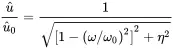
Amplitude and phase resonance occur at the same frequency ω 0. At resonance the viscously damped system amplification is u^/u^0=1/2ζ. Hence
 (1.66)
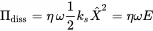
There is a further interpretation of the loss factor. ΔEcycle is the energy dissipated per cycle. The dissipated power given by Πdiss=ΔEd/T=ΔEcycleω/2π. Using equations ( 1.57) and ( 1.61) we get:
 (1.67)
At the beginning of the cycle the total energy E is stored as potential energy in the spring. The dissipated power is a product of damping loss, frequency and the total energy of the system. This will be frequently used in the following sections, but particularly in Chapter 6about statistical energy methods. The energy aspect leads to an equivalent definition of the loss factor:
 (1.68)
Thus, the damping loss factor can be seen as the criteria, defining the relative loss of energy per cycle divided by 2 π . In this zoo of damping criteria we have related c v, ζ , c vc, η , Δω, τ and Q . Table 1.1summarizes those quantities and puts them in relation to the others.
Table 1.1 Relation of important damping criteria
| Name | Symbol | cv,cvc | ζ | η | Q | Δω | τ |
|---|---|---|---|---|---|---|---|
| Viscous damping | c v | 1 | ζcvc | ||||
| Critical damping ratio | ζ | cv/cvc | 1 | η/2 | 12Q | Δω/2ω0 | 1/ω0τ |
| Critical damping | c vc | 4mks | 2ζmω0 | ||||
| Damping loss | η | 2cv/cvc | 2 ζ | 1 | 1/Q | Δω/ω0 | 2/ω0τ |
| Qualtity factor | Q | ccv2cv | 12ζ | 1/η | 1 | ω0Δω | ω0τ2 |
| 3dB bandwidth | Δω | 2ζω0 | ηω0 | ω0/Q | 1 | 12τ | |
| Decay time | τ | 1/ζω0 | 2/ω0η | 2Q/ω0 | 2/Δω0 | 1 |
In tools and software for vibroacoustic simulations many different quantities are used. The overview of all those different criteria shall help to avoid mistakes and confusion.
1.3 Two Degrees of Freedom Systems (2DOF)
The harmonic oscillator is also named as single degree of freedom (SDOF) system. Realistic systems consist of multiple degrees of freedom (MDOF). In order to keep things manageable we stay in a first step with two degrees of freedom. As for the SDOF case several phenomena can be treated exemplarily, especially the coupling effects. For presenting the idea of MDOF systems the start is done by two degrees of freedom (2DOF). The equations of motion for such a system as shown in Figure 1.11 are
 (1.69)
 (1.70)
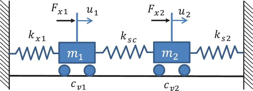
Figure 1.11 Two degrees of freedom system. Source : Alexander Peiffer.
By introducing harmonic motion for u1=u1ejωt and u2=u2ejωt we get
 (1.71)
 (1.72)
neglecting the time dependence ejωt. It is practical to write this in matrix form:
 (1.73)
In the following, the square brackets and the curly brackets denote a coefficient matrix and vector, respectively.
1.3.1 Natural Frequencies of the 2DOF System
We start with a simplified system without damping and external forces in order to get the natural frequencies of the system.
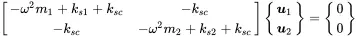 (1.74)
This equation can be rearranged so that it corresponds to the general eigenvalue problem
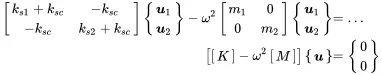 (1.75)
The non trivial solutions of this are given by:
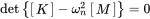 (1.76)
This leads to the characteristic equation with λ=ω2
 (1.77)
With ω12=ks1/m1, ω12=ks1/m1 and ωc2=ksc(m1+m2)m1m2 the solutions are:
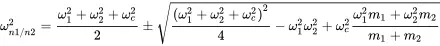 (1.78)
The eigenvalues shall be entered into the equations to solve for {Ψi}.
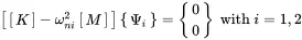 (1.79)
leading to the surprisingly simple eigenvalues after some painful math
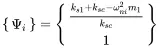 (1.80)
The results present the modes of the system or the shape of movement for this natural frequency. Let us simplify the above expression by additional conditions: ks1=ks2=ks and m1=m2=m.
So the modal frequencies read with ω02=ks/m
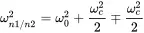 (1.81)
Интервал:
Закладка:
Похожие книги на «Vibroacoustic Simulation»
Представляем Вашему вниманию похожие книги на «Vibroacoustic Simulation» списком для выбора. Мы отобрали схожую по названию и смыслу литературу в надежде предоставить читателям больше вариантов отыскать новые, интересные, ещё непрочитанные произведения.


Обсуждение, отзывы о книге «Vibroacoustic Simulation» и просто собственные мнения читателей. Оставьте ваши комментарии, напишите, что Вы думаете о произведении, его смысле или главных героях. Укажите что конкретно понравилось, а что нет, и почему Вы так считаете.