Alexander Peiffer - Vibroacoustic Simulation

The mode shapes are orthogonal as can be derived by assuming two different solutions m,n

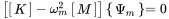(1.106)

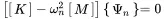(1.107)

Multiplying ( 1.107) from the left with the transposed {Ψm}T gives

(1.108)

Transposing ( 1.106) and multiplying from the right with {Ψ}n reads as

(1.109)

The difference between ( 1.108) and ( 1.109) leads to

(1.110)

Since ωn2≠ωm2 this requires

(1.111)

Using this in Equation ( 1.109) gives also

(1.112)

Thus, the mode shapes are orthogonal to each other with respect to [K] and [M]. For normalisation we multiply ( 1.106) from the left with {Ψ}m

(1.113)

and get

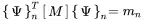(1.114)

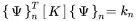(1.115)

for the modal mass m nand stiffness k nwith the following relation to the modal frequency

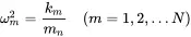(1.116)

The orthogonality of the mode shapes allows using them as a base for new coordinates that will simplify or condense the equation of motion. It is convenient to chose a normalisation with modal mass unity, thus mn=1, hence:

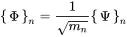(1.117)

{Φ}n is called the mass-normalized mode shape of the system. With Equation ( 1.116) and writing the mass normalized modes in matrix form

(1.118)

it becomes clear that the normalisation from ( 1.114) and ( 1.115) now reads as follows:

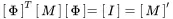(1.119)

(1.120)

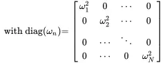(1.121)

The prime (′) denotes modal coordinates or matrices and [I] is the unit matrix. Due to the orthogonality of the modes every solution qcan be expressed as

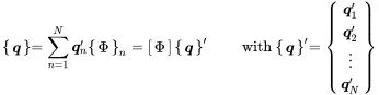(1.122)

and

(1.123)

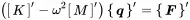
The vector {q′} with components qn′ is the displacement in modal coordinates. coordinates ! modal Entering this into ( 1.103) and multiplication from the left with [Φ]T provides

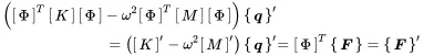(1.124)

Fn′ are the components of the modal force vector F′. Using the above defined orthogonality and normalisation we get:

(1.125)

or in another form:

(1.126)

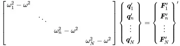
The response shape is reconstructed using ( 1.122). Thus, with modal coordinates expressed by independent degrees of freedom – the modes – the system decouples. This can by seen by the diagonal form of the matrix. For a system with N degrees of freedom, the modal solution is exact. The similarity to Equation ( 1.28) underlines that every mode can be interpreted as a single resonator. Thus, every dynamical system can be interpreted as a group of independent resonators of modal mass m nand stiffness ωn2mn In accordance with Equation ( 1.63) we may introduce a modal damping η nfor every mode. In that case the response in modal coordinates is:

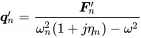(1.127)

In computational dynamics the solution of the homogeneous equation for normal modes and the calculation of the system response using the diagonal form is called modal frequency response . Finite element methods are frequently applying this method to simplify the solution and to condense the system equations to a reduced coordinate system. In addition modes are an excellent option to exchange model information or simulation results between different solvers. Usually, the modal base is truncated and not all modes are considered. In that case the modal solution is only an approximation of the direct solution. The denominator ωn2−ω2 reveals that the participation of every mode to the global solution decreases with the distance from the modal frequency. Thus, a reasonable set of modes near the frequency of interest can by sufficient.

Finally, we conclude that the change in the coordinate base to modal coordinates keeps the general format of the equation of motion.

(1.128)