Alexander Peiffer - Vibroacoustic Simulation

(1.140)

Let us consider that the process g is linked to f by a linear factor K :

The error or deviation of this assumption reads

(1.141)

or in terms of the mean square value

(1.142)

This can be rewritten as

(1.143)

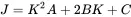
This is a minimization problem and we search for the slope K that minimizes the sum of squared deviations J . This function has a quadratic dependence and can be rewritten as

(1.144)

where A=E[f2], B=−E[fg], and C=E[g2], with all three terms being real expected values from real random processes. Equation ( 1.143) is parabolic in shape, and the minimum is found by setting the first derivative with respect to K to zero.

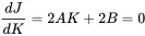(1.145)

Therefore, the point that minimizes J is given by K0=−B/A. In order to assure K 0being a minimum we need d2J/dK2>0, meaning that A must be positive. This can be easily proven, as the expected value of the squared function E[f2] must be positive. If we substitute K 0into Equation ( 1.143) we get the following relationships for K 0and J 0

(1.146)

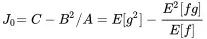(1.147)

Using the definition of variances we can write J 0in the case of zero mean processes in a non-dimensional form:

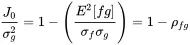(1.148)

The quantity ρfg=E[fg]/σfσg is the normalized correlation coefficient correlation coefficient ! normalised between f and g . If both processes are perfectly correlated ρfg=1. If they are fully uncorrelated ρfg=0. In terms of the linear relationship from ( 1.141) all points would be perfectly on the line for full correlation and would be arbitrarily distributed for no correlation (Figure 1.22).

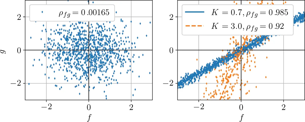
Figure 1.22 Example for correlation of random processes. No correlation (left) and different correlation values (right). Source : Alexander Peiffer.

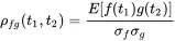
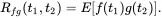
In the above considerations we have taken the values from an ensemble of random processes or signals taken at t 1. We can also define a correlation coefficient for values taken from two processes at different times t 1and t 2:

(1.149)

The numerator is called the cross correlation function cross correlation:

(1.150)

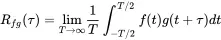
If the two processes are stationary the value of the cross correlation function depends only on the distance between the two times, i.e. t2=t1+τ. τ is called the lag or separation between the two time samples and we can write:

(1.151)

It also makes sense to correlate the function f ( t ) with itself at later moments f(t+τ). This is called the autocorrelation function defined by:

(1.152)

This function will later enable us to describe the spectrum of random functions. At τ = 0 the value is known as variance of f ( t ) as given by Equation ( 1.137):

(1.153)

The autocorrelation is symmetric in time, proven by:

(1.154)

In addition some useful properties can be derived for the cross correlation function

(1.155)

So we get finally

(1.156)

For the stationary ergodic process we can replace the ensemble averaging by the average over time

(1.157)

The Fourier transform of a random signal would lead to infinite results because it is not approaching zero. Fourier series cannot be applied too, because there is no periodicity in the signal. A smart solution is to use the correlation function for the Fourier transform and not the random signal itself. The correlation is a decaying function that is suitable for infinite integration due to the 1/T factor in ( 1.157). We start with the pair of Fourier transforms of the autocorrelation:

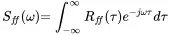(1.158a)

(1.158b)

Sff(ω) is called the auto spectral density auto spectral density of the signal f ( t ). It is a measure of how the signal energy is distributed over the frequency range. This becomes quite obvious if we look at τ = 0 and use ( 1.153):