Alexander Peiffer - Vibroacoustic Simulation

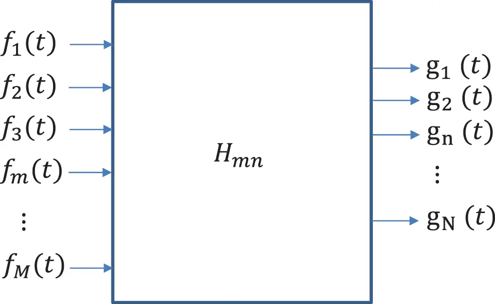
Figure 1.24Multiple-input–multiple-output (MIMO) system. Source : Alexander Peiffer.

The linear system function is described by M × N functions Hmn(ω) in frequency domain or hmn(τ) in time domain. The response of the m th output channel in time domain is given by

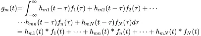(1.195)

In the frequency domain, in the response at output m the convolution is replaced by multiplication

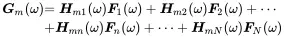(1.196)

Both equations can be written in matrix form. The frequency domain matrix reads as

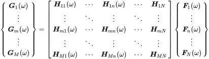(1.197)

or in short form

(1.198)

The force excitation and displacement response matrix [H(ω)] corresponds to the inverse dynamic stiffness matrix of Equation ( 1.83).

The contemplations in section 1.6.3 dealt with a single random input of one system. The cross spectrum or correlation was only applied to input and output. Imagine a system that has many sources that have random nature. In the case of a car this could be the exhaust noise, the cooling ventilation, and the engine. The noise linked to the stroke movement will be correlated to the component that is transmitted via the muffler to exhaust, whereas the flow noise generated by the turbulent flow in the muffler is not correlated to the stroke harmonics. Thus, in practical vibroacoustic systems there is a mix of sources that are correlated to each other. Some are independent – thus uncorrelated – and some are a mix of both, as the discussed exhaust example.

Equations ( 1.196) and ( 1.195) can only be used in case of fully correlated input because each summand in those equations will have a different phase or time delay for each set of input signals taken from the ensemble of possible input or for each separate test.

Consider a set of N random input signals as given in Equation ( 1.195) or ( 1.196). For the description of the input we need the power spectral density or autocorrelation of all signals fn(t) given by

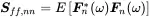(1.199)

Here the index ff denotes that only the input is considered, and nn that it is the autocorrelation of the n th input. In addition the cross correlation between the input signals is given by:

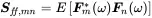(1.200)

This expression is called the cross spectral density matrix that looks in large form

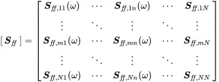(1.201)

This is a hermitian matrix due to the symmetry relationship of cross spectra also following from the expected value of each spectral product

(1.202)

For further considerations it is helpful to write the cross spectral matrix using the input spectra in vector form. Because of the matrix multiplication notation – row times column – the cross spectral density matrix can be written as

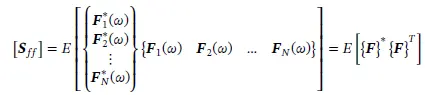(1.203)

In some literature on hybrid theory the complex conjugate of the cross spectral density matrix is used

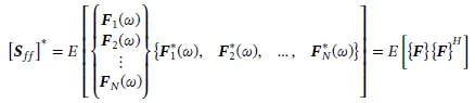(1.204)

It is helpful to understand how the matrix coefficients look for the following extreme cases:

Fully uncorrelated signals

Fully correlated signals.

The hermitian operator ⋅H is used, which combines the operations of complex conjugation and transposition.

Fully uncorrelated input signals mean that the cross correlation is zero. A model of this is the “rain-on-the-roof” excitation because each drop falls fully independent from its brother drops on the roof. This means that the cross correlation matrix has only diagonal components. All off-diagonal components are zero.

In this case the signals are correlated and have a clear phase relationship to a reference. Thus, all signals are linearly dependent to this reference. So every column of the cross spectral matrix can by derived by a linear combination of the other columns. So, we don’t need the full matrix and Equation ( 1.198) can be applied.

When the input can only be defined by a cross spectral matrix [Sff], the same is true for the response Gm(ω).

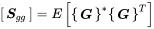(1.205)

with

and so

(1.206)

The system matrix Hcan be removed from the expected value operator

(1.207)

and finally

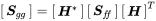(1.208)

This expression determines the cross spectral response of a linear MIMO system excited by random load. Typical numerical system equations have millions of degrees of freedom. Therefore, in many cases the above equation cannot by used straightforwardly, because this would lead to triple multiplication of Hermitian-but-huge matrices. Thus, for random excitation we need different approaches for the response calculation. The conjugate version of Equation ( 1.208) is

(1.209)