Alexander Peiffer - Vibroacoustic Simulation

The product of Fourier transforms corresponds to a convolution in time domain ( 1.42), hence:

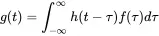(1.174)

or alternatively, as

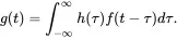(1.175)

A system is called causal (and this is definitely the case for any mechanical system) when the impulse response is zero at times smaller than zero (it can only react when it has experienced an excitation), so

(1.176)

That means we can rearrange the integration limits as follows:

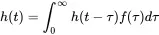(1.177)

All those forms are convolution integrals according to ( 1.46) and the response can be written as

(1.178)

So, with this function we can express any response of a linear system using the above convolution integral. When considering a unit frequency excitation F(ω)=1 Equation ( 1.173) shows that the response equals the transfer function.

(1.179)

The inverse Fourier transform of the unit spectrum ejωt0=1 for t0=0 is the delta function δ(t) according to ( 1.32). In the time domain this reads as the following convolution integral

(1.180)

We see that the transfer function in time domain is the response of the system to a delta function. Consequently, this function is called the impulse response of the system. When we calculate the inverse Fourier transform of the frequency response function of the damped harmonic oscillator we get as impulse response function

(1.181)

This is the solution of the following equation of motion

(1.182)

which corresponds to the solution of the homogeneous version in ( 1.1) for the following initial conditions

(1.183)

Finally, with the definition of system response functions in time and frequency domain, there is a powerful description available. This will be used in Section 1.6.3 in order to describe the system response to random signals.

We know from section 1.5.4 that the random signal cannot be Fourier transformed. As a consequence we apply the correlation methods from above to the output of a system excited by random signals. We start with the autocorrelation of the system output g from excitation by random input f

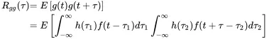(1.184)

The impulse response can by taken out from the expected value operation, because it does not depend on the time. Hence we get

(1.185)

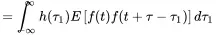
When we assume a retarded time argument of τ′=τ+τ1−τ2 the expected value can be interpreted as the autocorrelation of f ( t ). With this assumption we get:

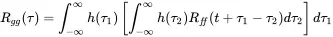(1.186)

The term in the rectangular brackets can be seen as the convolution with argument (τ+τ1).

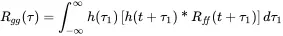(1.187)

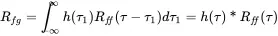
By replacing τ 1by − u this reads as

(1.188)

using that Rff(τ) is symmetric in τ . This equation can be converted into frequency domain using the fact that time reversal in time corresponds to complex conjugate spectra:

(1.189)

So we know now the autospectrum of the system excited by random response. Next we investigate the cross correlation between input and output.

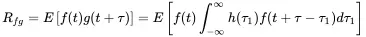(1.190)

(1.191)

This expression can be simplified by assuming the expected value to be the auto-convolution with argument τ−τ1 to:

(1.192)

Converting this into the frequency domain gives:

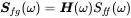(1.193)

This is a very important result: every transfer function (also using deterministic signals) can be determined by the ratio of the cross spectrum to auto spectrum.

(1.194)

In principle this can also be done by using the Fourier transform ( 1.173), using time-limited excitation and dividing output and input FT, but the cross spectral variant is much more robust against measurement noise.

Mechanical set-ups with multiple degrees of freedom are multiple-input–multiple-output (MIMO) systems. The frequency response is determined by matrix inversion or solution of the matrix as shown in Equation ( 1.83)

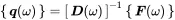
In a more general form a MIMO system is defined as a system with N input signals fn(t) and M output signals gm(t).