Alexander Peiffer - Vibroacoustic Simulation

1 Julius S. Bendat and Allan G. Piersol. Engineering Applications of Correlation and Spectral Analysis. Wiley, New York, 1980. ISBN 978-0-471-05887-8.

2 Cyril M. Harris and Charles E. Crede. Shock and Vibration Handbook. McGraw-Hill, New York, NY, U.S.A., second edition, 1976. ISBN 0-07-026799-5.

3 P. A. Nelson and S. J. Elliott. Active Control of Sound. Academic, London, 1993. ISBN 0-12-515426-7.

1 1 In this book the convention ejωt for the complex harmonic function is used. Literature that deals with wave propagation often use e−jωt to have positive wavenumber for positive wave propagation. However, as in every textbook in acoustics I denote the used convention on the first page to avoid confusion.

The acoustic wave motion is described by the equations of aerodynamics that are linearized because of the small fluctuations that occur in acoustic waves compared to the static state variables. The fluid motion is described generally by three equations:

Continuity equation – conservation of mass

Newton’s law – conservation of momentum

State law – pressure volume relationship.

For lumped systems the velocity is simply the time derivative of the point mass position in space. The same approach can be used in fluid dynamics, but here the continuous fluid is subdivided into several cells and their movement is described by trajectories. This is called the Lagrange description of fluid dynamics. Even if the equation of motions are simpler in that formulation it is quite complicated to follow all coordinates of fluid volumes in a complex flow. Thus, the Euler description of fluid dynamics is used. In this description the conservation equations are performed for a control volume that is fixed in space and the flow passes through this volume.

In this chapter, the three dimensional space is given by the Cartesian coordinates x={x,y,z}T and the velocity of the fluid v={ vx, vy, vz }T.

For simplicity we consider first the flow in the x-direction as in Figure 2.1. The mass flow balance contains the following quantities:

1 The elemental mass m=ρdV=ρA with A=dydz.

2 Mass flow into the volume (ρvxA)x.

3 Mass flow out of the volume (ρvxA)x+dx.

4 Mass input from external sources m˙.

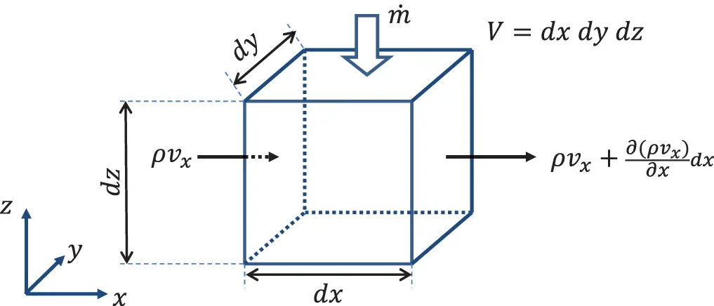
Figure 2.1 Mass flow in x-direction through control volume. Source : Alexander Peiffer.

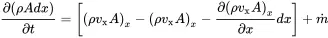
leading to equation

(2.1)

for mass conservation. Expanding the second term on the right hand side in a Taylor series gives

and finally

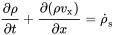(2.2)

This one dimensional equation of mass conservation in x-direction can be extended to three dimensions:

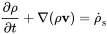(2.3)

The second term of ( 2.3) may be confusing, but it says that the change of density is not only determined by a gradient in the velocity field but also by a gradient of the density.

The same procedure is applied to the momentum of the fluid. As shown in Figure 2.2 we get for flow in x-direction:

1 The momentum of the control volume is ρvxdV=ρvxAdx.

2 The momentum flow into the volume (ρvx2A)x.

3 mass flow out of the volume (ρvx2A)x+dx.

4 The force at position x is (PA)x.

5 The force at position x+dx is (PA)x+dx.

6 External volume force density fx.

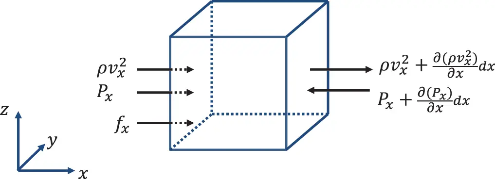
Figure 2.2 Momentum flow in x-direction through control volume. Source : Alexander Peiffer.

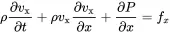
Thus, the conservation of momentum in x reads

(2.4)

Using Taylor expansions for (ρvx2A)x+dx and (PA)x+dx gives

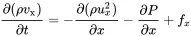(2.5)

Here, fx=Fx/(Adx) is the volume force density (force per volume). Using the chain law the partial derivatives of the first and second term lead to

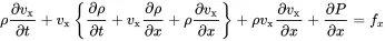(2.6)

The term in brackets is the homogeneous continuity Equation ( 2.1), and Equation ( 2.6) simplifies to

(2.7)

As with the conservation of mass, this can be extended to three dimensions:

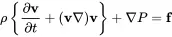(2.8)

This equation is the non-linear, inviscid momentum equation called the Euler equation.

The above equations relate pressure, velocity and density. For further reducing this set we need a third equation. The easiest way would be to introduce the . Here we start with the first law of thermodynamics in order to show the difference between isotropic (or adiabatic) equation of state and other relationships.

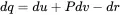(2.9)

With the following specific quantities per unit mass

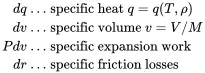(2.10)

With the specific entropy ds=dq+drT we get:

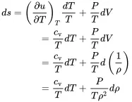(2.10)

The relation dv=d(1/ρ) comes from the fact that v is a mass specific value and therefore the reciprocal of the density ρ=1/v. For an ideal gas we have

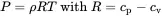(2.11)

cp and cv are the specific thermal heat capacities for constant pressure and volume, respectively. That is the ratio of temperature change ∂T per increase of heat ∂q. From the total differential