Alexander Peiffer - Vibroacoustic Simulation
Здесь есть возможность читать онлайн «Alexander Peiffer - Vibroacoustic Simulation» — ознакомительный отрывок электронной книги совершенно бесплатно, а после прочтения отрывка купить полную версию. В некоторых случаях можно слушать аудио, скачать через торрент в формате fb2 и присутствует краткое содержание. Жанр: unrecognised, на английском языке. Описание произведения, (предисловие) а так же отзывы посетителей доступны на портале библиотеки ЛибКат.
- Название:Vibroacoustic Simulation
- Автор:
- Жанр:
- Год:неизвестен
- ISBN:нет данных
- Рейтинг книги:3 / 5. Голосов: 1
-
Избранное:Добавить в избранное
- Отзывы:
-
Ваша оценка:
Vibroacoustic Simulation: краткое содержание, описание и аннотация
Предлагаем к чтению аннотацию, описание, краткое содержание или предисловие (зависит от того, что написал сам автор книги «Vibroacoustic Simulation»). Если вы не нашли необходимую информацию о книге — напишите в комментариях, мы постараемся отыскать её.
Learn to master the full range of vibroacoustic simulation using both SEA and hybrid FEM/SEA methods Vibroacoustic Simulation
Vibroacoustic Simulation
Vibroacoustic Simulation
Vibroacoustic Simulation — читать онлайн ознакомительный отрывок
Ниже представлен текст книги, разбитый по страницам. Система сохранения места последней прочитанной страницы, позволяет с удобством читать онлайн бесплатно книгу «Vibroacoustic Simulation», без необходимости каждый раз заново искать на чём Вы остановились. Поставьте закладку, и сможете в любой момент перейти на страницу, на которой закончили чтение.
Интервал:
Закладка:
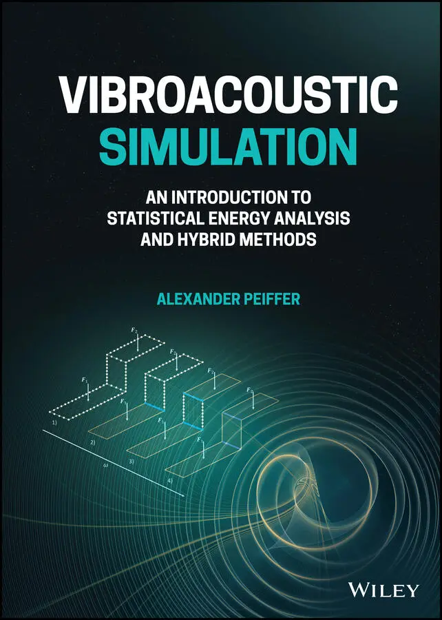
 (2.12)
we can derive
 (2.13)
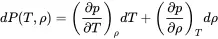
Using all above relations the change in density dρ is:
 (2.14)
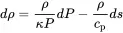
with κ=cv/cp. In most acoustic cases the process is isotropic: i.e. time scales are too short for heat exchange in a free gas; thus ds=0, and the change of pressure per density is
 (2.15)
In case of constant temperature (isothermal) dT=0 we get with ( 2.12) and the ideal gas law ( 2.11):
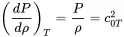 (2.16)
As we will later see, c0 is the . Newton calculated the wrong speed of sound based on the assumption of constant temperature that was later corrected by Laplace by the conclusion that the process is adiabatic. For fluids and liquids like water a different quantity is used because there is no such expression as the ideal gas law. The bulk modulus is defined as:
 (2.17)
Due to ( 2.15) and ( 2.16) the relationship between the bulk modulus K and c0 is:
 (2.18)
The bulk modulus can be defined for gases too, but we must distinguish between isothermal or adiabatic processes.
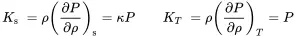 (2.19)
2.2.4 Linearized Equations
Equations ( 2.3) and ( 2.8) can be linearized if small changes around a certain equilibrium are considered:
 (2.20)
 (2.21)
 (2.22)
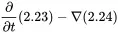
Inserting ( 2.22) into the equation of continuity ( 2.3), neglecting all second order terms as far as source terms, and setting 1v0=0 the linear equation of continuity is:
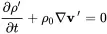 (2.23)
Doing the same for the equation of motion ( 2.8) leads to:
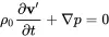 (2.24)
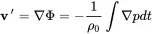
Using the curl(∇×) of this equation it can be shown that the acoustic velocity v′ can be expressed using a so-called velocity potential which will be useful for the calculation of some wave propagation phenomena.
 (2.25)
2.2.5 Acoustic Wave Equation
From the following operation
follows
 (2.26)
With the equation of state ( 2.15) for the density we get the linear wave equation for the acoustic pressure p
 (2.27)
Inserting the velocity v′=∇Φ derived from the potential Φ into the linear equation of motion ( 2.24) provides the required relation between pressure and the velocity potential
 (2.28)
Thus, the relationship between pressure p and the velocity potential Φ is
 (2.29)
Entering this into the wave equation ( 2.27) and eliminating one time derivative gives:
 (2.30)
The definition of the velocity potential ( 2.25) and equation ( 2.29) can be applied for the derivation of a relationship between acoustic velocity and pressure:
 (2.31)
2.3 Solutions of the Wave Equation
In acoustics we stay in most cases in the linear domain, so we change the notations from equations ( 2.20)–( 2.22):
 (2.32)
Equations ( 2.27) and ( 2.30) define the mathematical law for the propagation of waves. For the explanation of basic concepts the wave equation is used in one dimensional form.
2.3.1 Harmonic Waves
According to D’Alambert every function of the form p(x,t)=Af(x−c0t)+Bg(x+c0t) is a solution of the one-dimensional wave equation. In the following we will consider harmonic motion or waves so we replace the functions f and g by the exponential function with
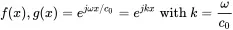 (2.33)
and get
 (2.34)
The first term of the right hand side of this equation is travelling in positive directions, the second in negative directions 2. Harmonic waves are characterized by two quantities, the angular frequency ω and the wavenumber k. The first is the frequency (in time) as for the harmonic oscillator, and the second is a frequency in space. A similar relationship can be found between the time period T and the wavelength λ. Space and time domains are coupled by the sound velocity c0 as shown in Table 2.1.
Table 2.1 Quantities of wave propagation in time and space domains.
| Name | Time | Space | ||
|---|---|---|---|---|
| Symbol | Unit | Symbol | Unit | |
| Period | T | s | λ=c0T | m |
| Frequency | f=1T | s −1(Hz) | (⋅)=1λ | m −1 |
| Angular frequency | ω=2πf=2πT | s −1 | k=2πλ=ω/c0 | m −1 |
The time integration in Equation ( 2.31) corresponds to the factor 1/(jω) and reads in the frequency domain:
Читать дальшеИнтервал:
Закладка:
Похожие книги на «Vibroacoustic Simulation»
Представляем Вашему вниманию похожие книги на «Vibroacoustic Simulation» списком для выбора. Мы отобрали схожую по названию и смыслу литературу в надежде предоставить читателям больше вариантов отыскать новые, интересные, ещё непрочитанные произведения.


Обсуждение, отзывы о книге «Vibroacoustic Simulation» и просто собственные мнения читателей. Оставьте ваши комментарии, напишите, что Вы думаете о произведении, его смысле или главных героях. Укажите что конкретно понравилось, а что нет, и почему Вы так считаете.