Alexander Peiffer - Vibroacoustic Simulation

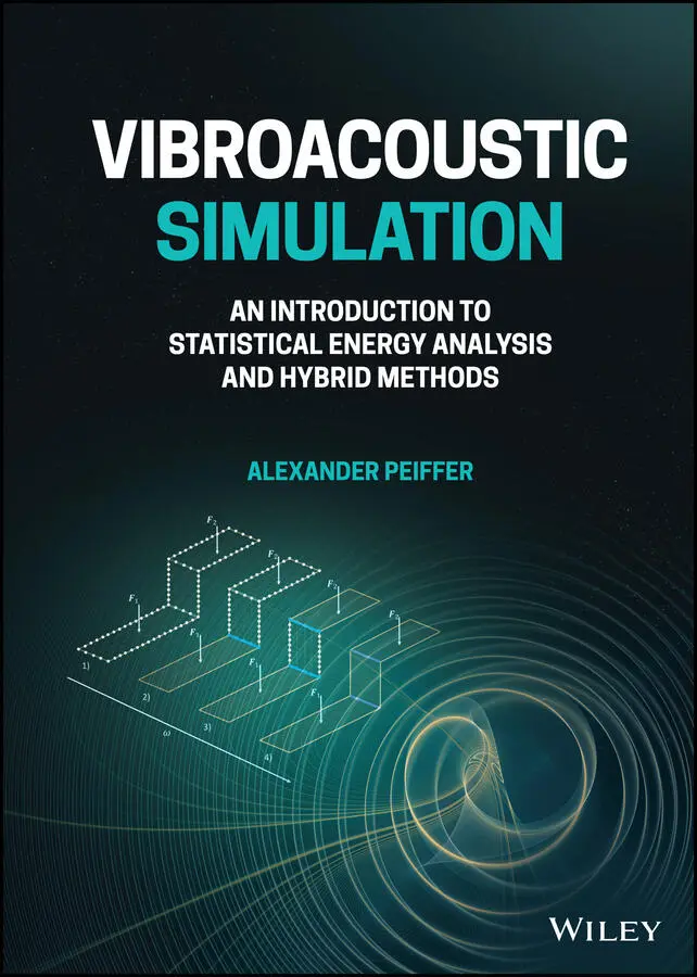
(1.159)

The autocorrelation is a real symmetric function, thus the auto spectrum as Fourier transform of this is a symmetric real valued function in frequency.

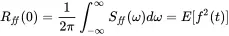
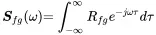
We define the cross spectral density function as the Fourier transform of the cross correlation function from Equation ( 1.151) and the back transformation:

(1.160)

(1.161)

Changing the integration constant τ=−τ′ and using symmetry ( 1.156) reveals

(1.162)

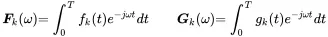
Mathematically, the expected value of an ergodic processes is derived by the investigation of infinite time periods. However, this can neither be realized in tests nor numerical simulations. We are restricted to specific time slots, so let us assume the Fourier transform of two random signals f ( t ) and g ( t ).

(1.163)

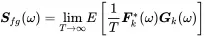
It can be shown by a straightforward but lengthy proof by Bendat and Piersol (1980) that the cross spectral density is a complex function given by

(1.164)

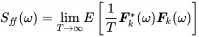
Here, we take the signals of infinite duration from an ensemble of recordings. The same can be shown for the autospectrum.

(1.165)

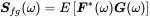
So these important relationships show, that if we have an infinite time period T and we average over a whole ensemble of such records we can determine the auto and cross spectra from this. In practical test and simulation situations we will see that for a given number of time signals of finite time T we can estimate the power- and cross spectral density. For convenience we abbreviate Equation ( 1.164)

(1.166)

Note that the cross correlation Rfg(τ) of time signals f ( t ) and g ( t ) can be reconstructed from the inverse Fourier transform.

As shown in section 1.5.4 and Equation ( 1.164) the expected value of the Fourier transform of an ensemble of signals of infinite duration is given by:

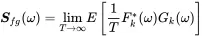
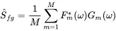
It is helpful to convert this into an expression for a finite number of signals of finite duration. Usually, there is one signal of time length T available that is separated into M partitions of length T w. So the estimate would be:

(1.167)

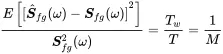
In Bendat and Piersol (1980) it is shown that the relative error is given by:

(1.168)

So for a given time length T the more we average, the more precise is the spectral estimate, but we sacrifice spectral resolution against statistical precision.

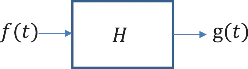
Figure 1.23Sketch of a single-input–single-output system. Source : Alexander Peiffer.

Any car, building, air plane or machine represents a dynamic system. This dynamic system is excited by source function f ( t ), e.g. a force. The excitation is called the input of the system. This excitation leads to a specific response g ( t ) called the output of the system. The simplest cases are systems with one input and output, e.g. the forced harmonic oscillator. Those systems are called single-input–single-output systems (SISO). Real systems are usually driven by multiple inputs or sources and have continuous or multiple responses. Those are called multiple-input–multiple-output systems (MIMO). Every system is described by its transfer function: i.e. a functional expression H that relates the inputs to the outputs.

(1.169)

The practical advantage of such a formalism is that a complex realistic system is reduced to the quantities of interest. All intermediate steps of sound and vibration prediction are neglected. A practical example would be the force from the engine mount as input exciting the car system. A reasonable output could be the sound pressure at the drivers ear.

We restrict our considerations to linear systems. Thus, the response of the system to the sum of two signals f1(t) and f2(t) is given by the sum of each single response

(1.170)

If the inputs are multiplied by constants a and b the responses scale linearly with the input

(1.171)

This is called the superposition principle.

The Equation ( 1.28) for the displacement response of the damped harmonic oscillator

(1.172)

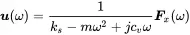
is an example for a system response in frequency domain. With uand F sas complex amplitudes of harmonic signals we can express the system properties easily in the frequency domain

(1.173)

Thus, H(ω) is the system transfer function in frequency domain. It is usually a complex function.