Alexander Peiffer - Vibroacoustic Simulation

As clean harmonic signals are rare in technical systems we need a mathematical toolbox to deal with nonharmonic signals. Due to the Fourier theory (Nelson and Elliott, 1993) every deterministic time signal can be synthesized by a sum of harmonic components. This provides a theoretical link between periodic and harmonic but also transient signals. See appendix A. 1for a brief introduction.

The same theory can also be applied to stochastic or random signals but in a slightly different manner. Fourier analysis and methods for investigating the random processes and the description of mechanical systems by impulse response or frequency response functions is an important toolset for the description of vibroacoustic systems. In addition and due to digitalisation most signals or spectra are given as a discrete, digital set of values. This discrete formulation creates some pitfalls that may also lead to misinterpretations. Even though the signal analysis is not a major subject in vibroacoustic simulation it is a very important especially when acoustic experiments are performed.

Signals from technical processes are often not predictable and are generated randomly like pressure fluctuations in a turbulent flow, the impact of raindrops on a roof, or the stochastic combustion in a jet. For dealing with such signals the above described methods must be adapted. In addition we need formulations that allow for the definition of the statistics of random processes as there is no deterministic functionality between time or frequency and the physical quantity, for example force or displacement.

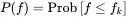
Imagine a random process creating signal sequences as shown in Figure 1.19. At each time the signal value f ( t ) may be different and has a certain continuous value. One option to characterize this signal is to define the probability that the signal value is less or equal to a specific value f k. Thus we define a probability for f ( t ) to be less than or equal to f k

(1.129)

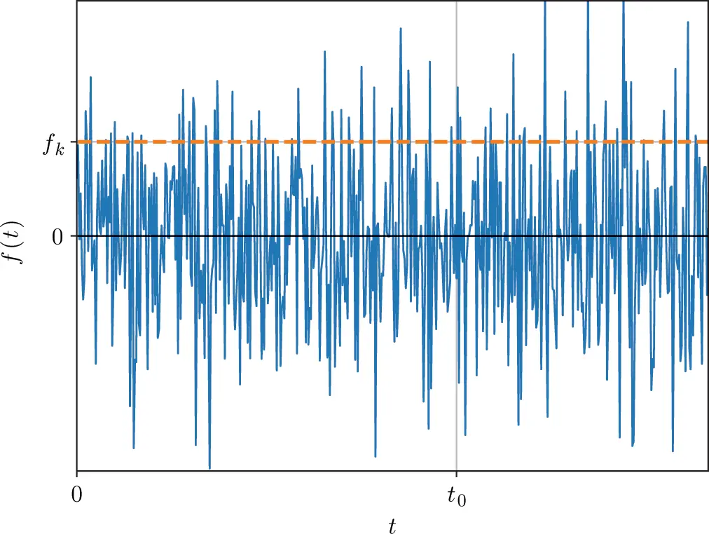
Figure 1.19 Stochastic fluctuation with time. Source : Alexander Peiffer.

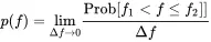
Next, we are interested in the probability that the value of f ( t ) is in a range defined by Δf=f2−f1 meaning the probability Prob[f1

(1.130)

Consequently in the limit Δf→0 the probability function density p is defined by

(1.131)

On the other side we can reconstruct the probability to be in the range of f 1to f 2by integrating over the probability density function

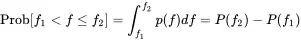(1.132)

In Figure 1.20 the examples for above defined functions are depicted. Those distinct ways of averaging reveal that the different averaging methods must be described in more detail. Until now averaging was performed over time intervals. This must not be confused with averaging over an ensemble. average averaging means averaging over an ensemble of experiments, systems, or even random signals. It will be denoted by ⟨⋅⟩E. Ensemble averaging can be similar to time averaging but this is only valid for specific time signals or random processes.

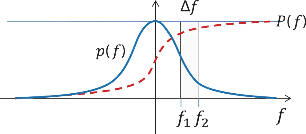
Figure 1.20 Probability and probability density function of a continuous random process. Source : Alexander Peiffer.

In Figure 1.21 the differences between time and ensemble averaging are shown. On the left hand side (ensemble) we perform a large set of experiments and take the value at the same time t 1, on the right hand side we perform one experiment but investigate sequent time intervals.

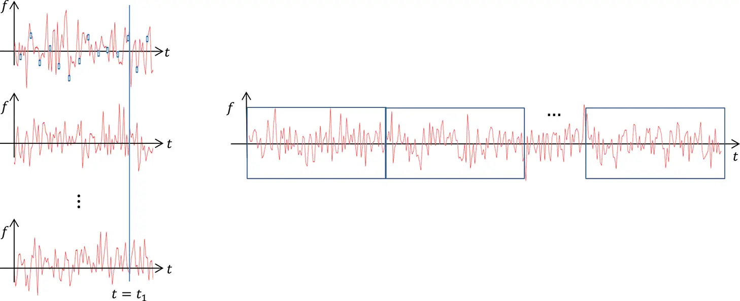
Figure 1.21 Ensemble and time averaging of signals from random processes. Source : Alexander Peiffer.

Consider now the mean value of an ensemble of N experiments. The mean value is defined by

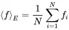(1.133)

If we assume N kdiscrete results f kthat occur with frequency rk=nk/N we can also write

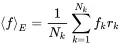
In a continuous form this can be expressed as rk=p(fk)Δfk

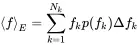(1.134)

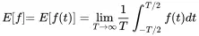
For fk→f we get the definition of the based on ensemble averaging and expressed as the integral over the probability density.

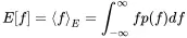(1.135)

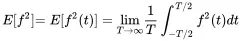
Similar to the expression for time signal rms-value, we define in addition the expected mean square value

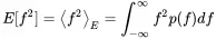(1.136)

and the variance

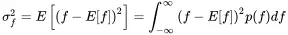(1.137)

We come back to the difference between ensemble and time averaging as shown in Figure 1.21. A process is called ergodic when the ensemble averaging can be replaced by time averaging, thus

(1.138)

(1.139)

We are usually not able to perform an experiment for an ensemble of similar but distinct experimental set-ups, but we can easily record the signals over a long time and take several separate time windows out of this signal.

Even more important than the key figures of one random process is the relationship between two different processes, the so-called correlation. It defines how much a random process is linearly linked to another process. Imagine two random processes f ( t ) and g ( t ). Without loss of generality we assume the mean values to be zero: