Alexander Peiffer - Vibroacoustic Simulation

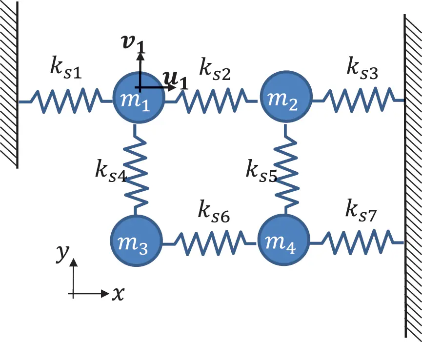
Figure 1.17 Multiple degrees of freedom network Source : Alexander Peiffer.

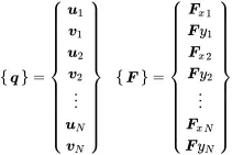
We speak about nodes for the different locations in space running over index i . Each node may have different degrees of freedom (DOF). In our case, there are two translational coordinates u and v . So the displacement and force vector is running over all DOF of all N nodes:

(1.90)

A recipe can be used to assemble the equations of motion in the above given matrix form. For this purpose we derive a set of rules that allows for creating those matrices. This is practical for the understanding of complex mechanical networks but also a good start for understanding the basics of finite element simulation which is also based on mathematical methods to create mass and stiffness matrices from a discretized model. The concept of nodes and DOF is also kept in the finite element simulation.

The mass matrix in multidimensional space follows from Newton’s law of point masses in free space.

(1.91)

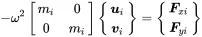
Using the complex amplitude notation of harmonic motion this leads to:

(1.92)

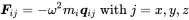
For every mass m iat node i the local mass matrix is depending on the available degrees of freedom for each mass node. For a two-dimensional system with {q}i={ui,vi}T we get:

(1.93)

The local matrices must by assembled for all degrees of freedom, so the system from Figure 1.17 will have the follwing mass matrix:

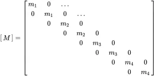(1.94)

A similar procedure is applied to the springs and the related stiffness matrix. Every spring k iconnects different points in space, so there are at least two nodes involved, unless the spring is connected to a rigid wall. Inspecting the spring in Figure 1.18 the force balance is:

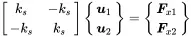(1.95)

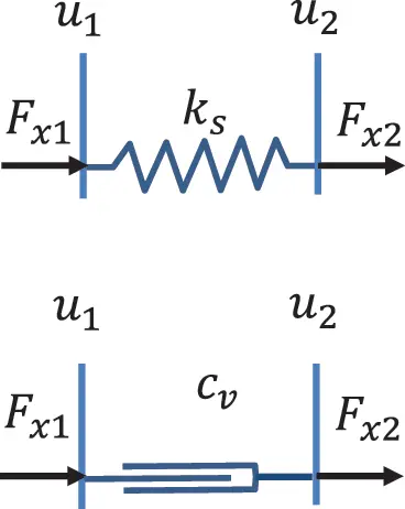
Figure 1.18 Spring and damper connection of two nodes. Source : Alexander Peiffer.

Springs connected to rigid walls are treated differently. In that case the DOF at the wall is constrained. Here for example u1=0, and we get for Equation ( 1.95)

(1.96)

If the spring is connected to the wall, only u 2changes with applied forces, and the reaction force in the constraint is −ksu2. Practically that is the reaction force that must be provided by the wall to keep the node in place. In the finite element terminology these constraints are called single point constraints (SPC).

The local matrices must be distributed among the global stiffness matrix [K]. For better visibility this is done for springs 2 and 4. The place of the local matrix of spring 2 in the global stiffness matrix follows from the u 1and u 2, the position of spring 4 from v 1and v 3.

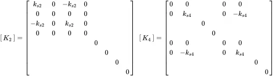(1.97)

For the system from Figure 1.17 and putting all free and constraint springs together we get:

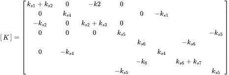(1.98)

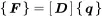
With this procedure the matrix formulation of the equation of motion can be created. A similar approach can be used if other elements like dampers are involved. Generally the local elements can be everything that can be expressed by a dynamic stiffness matrix [D(ω)] and can be added into a global matrix, independent from the fact if it comes from other models, simulation or test.

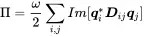
The power introduced into the MDOF system is calculated according to ( 1.49).

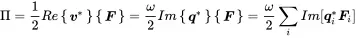(1.99)

The input power can be reconstructed from the dynamic stiffness matrix ( 1.89). We know that

(1.100)

hence

(1.101)

or in matrix notation

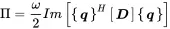(1.102)

Modes are natural shapes of vibration for a dynamic system. For a given excitation it would be of interest to see how well each mode is excited. In addition, these considerations lead to a coordinate transformation that simplifies the equations of motion.

We start with the discrete equation of motion in the frequency domain ( 1.89) and set the damping matrices [C] and [B] to zero

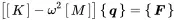(1.103)

Without external forces we get the equation for free vibrations, and we get the generalized eigenvalue problem

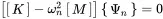(1.104)

The non-trivial solutions of this are determined by zero determinants

(1.105)

providing the modal frequencies ω n. Entering these frequencies and solving for Ψn provides the mode shape of the dynamic system. These are the natural modes (shapes) of vibration that occur at the modal frequencies.