Alexander Peiffer - Vibroacoustic Simulation

with the eigenvectors:

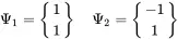
Thus, the first mode represents a uniform motion of both masses without any relative motion and thus no effect of the centre spring. The second mode is a symmetric resonance and the centre spring adds some extra stiffness leading to higher frequencies. See Figure 1.12 for both modes.

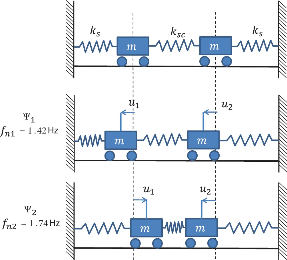
Figure 1.12 Mode shapes of the 2DOF example. Source : Alexander Peiffer.

When we enter numerical figures with m = 0.1 kg, ks=10 N/m and ksc=2 N/m we get the modal frequencies ωn1=10.0 s−1(fn1=1.59 Hz) and ωn2=11.83 s−1(fn2=1.88 s−1).

If the 2DOF system is excited by a force or a combination of several forces, the system of equations ( 1.73) is solved for every frequency. Equation ( 1.73) can by written in a more generic way

(1.82)

The solution can be written using the inverse of the stiffness matrix

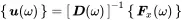(1.83)

This frequency response can be received for example by using numerical packages like MATLAB TM, Python (with NumPy) for a set of frequencies. In Figure 1.13 the response of the system for unit excitation of Fx1=1 N and Fx2=0 N is shown.

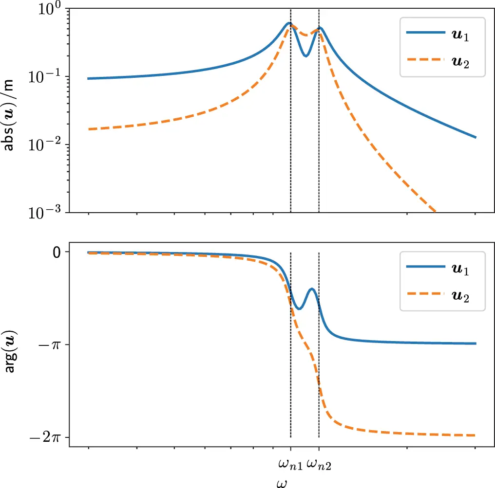
Figure 1.13 Magnitude and phase of response to unit force at mass 1. Source : Alexander Peiffer.

The harmonic oscillator can be an anti-vibration device. This is called a tuned vibration absorber (TVA) or dynamic vibration absorber (DVA) and is a kind of multi-purpose tool whenever you have to combat resonance issues. It is a very useful device if vibration at a particular frequency must be reduced. Many applications are single frequency cases as for example propeller harmonics. In addition DVAs are used for reducing the resonance effects under broadband excitation. Usually real technical systems have multiple resonances but the principle can be shown with a SDOF system as master system. In Figure 1.14 such a setup is shown. The exciting force can be for example a rotating or vibrating machinery.

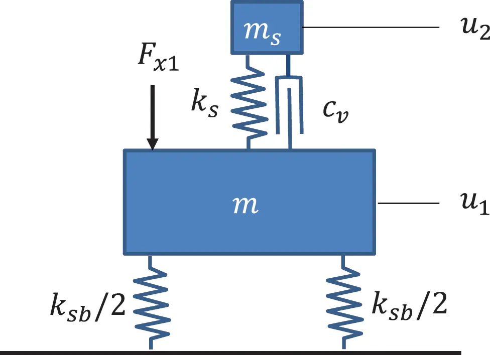
Figure 1.14 DVA mounted on resonant master system. Source : Alexander Peiffer.

The equation of motion is

(1.84)

with the following transfer function

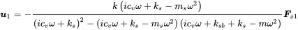(1.85)

The result is non-dimensionalized by dividing through the static response u1(0)=Fx1/ksb.

Assuming zero damping gives the characteristic equation for the combined resonances

(1.86)

With the resonance frequencies of each single system ω02=ksb/m, ωs2=ks/ms and the mass ratio μ=ms/m the resonance frequencies of the combined undamped system are given by

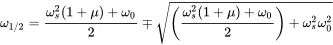(1.87)

Figure 1.15 shows the result for a master system with m = 0.1 kg and ksb=10 N/m and an additional DVA tuned to the same frequency as the master system with ms=0.02 kg and ks=2 N/m. Several curves for different critical damping ζ are given. From the undamped case we learn that the response can theoretically be reduced to zero but implicating two resonances at different frequencies. With additional damping the response can be diminished for a broad frequency range. The design of the best DVA is an optimisation task depending on several constraints as discussed in detail by Harris and Crede (1976). In the optimisation procedures issues such as total mass, DVA mass displacement, linearity range of the spring, and the dynamic must be considered.

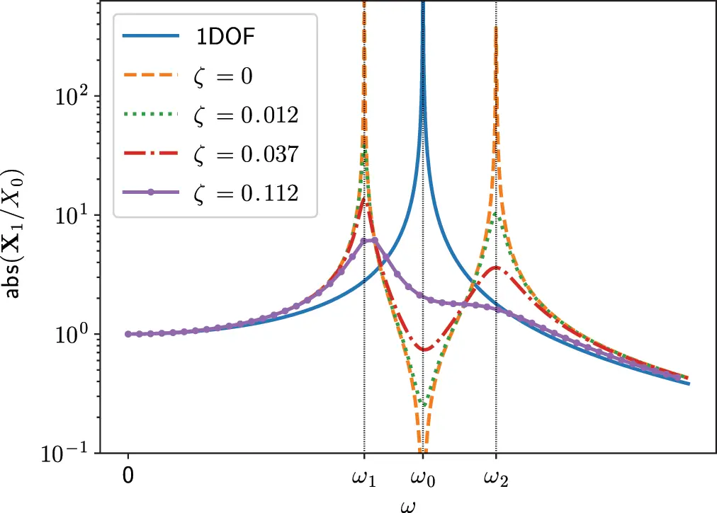
Figure 1.15 1DOF system with and without DVA. m = 0.1 kg, ms=0.02 kg, ksb=10 N/m, ks=2 N/m. Source : Alexander Peiffer.

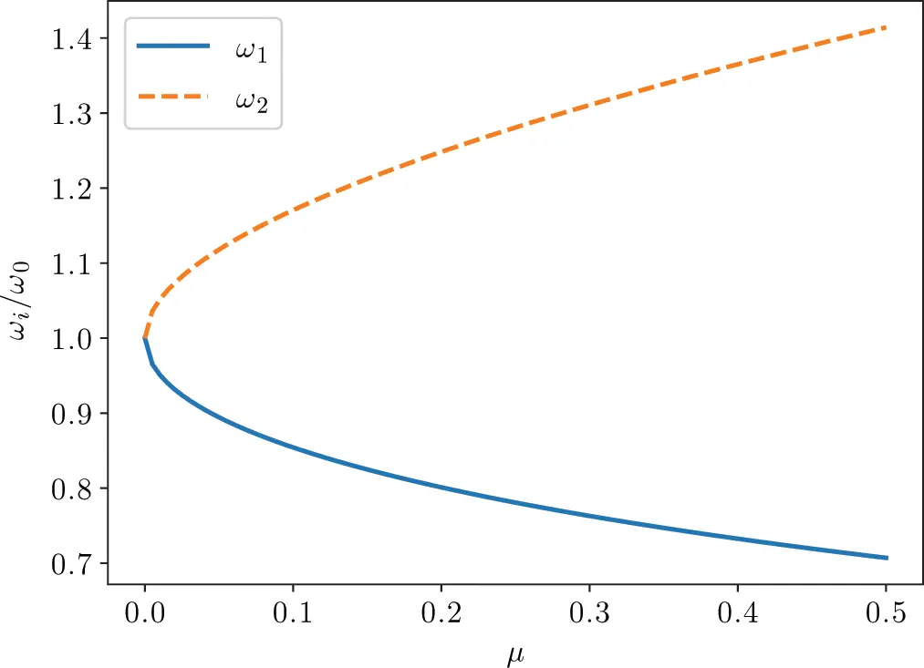
Figure 1.16Frequency spread for DVA tuned to the same frequency depending on mass ratio. Source : Alexander Peiffer.

The considerations above show the concept of how to write the equation of motion in matrix form. The matrices of the equation of motion in the frequency domain follow a certain convention in order to separate mass, stiffness and damping effects. As in Equation ( 1.73) the equation of motion of every discrete linear mechanical system can be approximated by the following form:

(1.88)

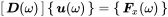
or in the frequency domain as

(1.89)

The coefficients q iof {q} are generic displacement degrees of freedom, for example the displacements u,v,w in x -, y - and z -directions at different positions. The first matrix [D] is called the dynamic stiffness matrix. The matrices in the parentheses are called mass matrix, damping matrix, stiffness matrix and proportional damping matrix. The solution of equation 1.89with regard to {q} is called frequency response.

The stiffness matrix must not be confused with the dynamic stiffness matrix. The dynamic stiffness matrix is frequency dependent and includes all matrices whereas the stiffness matrix includes the real and frequency independent stiffness part of the equation of motion. For specific lumped elements like springs and dampers there exist simple sub matrices that can be used to set up the global matrix of a more complex set-up. For illustration, see the example network of masses and springs in Figure 1.17.