Alexander Peiffer - Vibroacoustic Simulation

that is fluctuating for harmonic motion but with a net power flow.

For harmonic motion the power introduced into the system by a force Fx(t)=Fxejωt that generates the velocity response vx(t)=vxejωt is

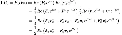(1.47)

The first term in the bracket is constant, the second oscillating with twice the excitation frequency. The first part is called active power and the second part the reactive. All introduced energy in one half cycle comes back in the next half cycle. The time average over one period leaves only the active part

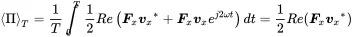(1.48)

The velocity can be expressed by the impedance V=Z/F or vice versa, so we get

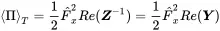(1.49)

The power considerations further clarify the naming conventions for the real and imaginary parts of the impedance. With Equation ( 1.40) the power introduced into the system equals Π=12|vx|2cv. Thus, the active power is controlled by the real part or resistance whereas the reactive part is determined by the imaginary component called reactance. The energy is dissipated in the resistive damping process, but power delivered to the reactive part goes into the kinetic and potential energy of mass and spring.

In many practical applications ζ is small and the amplitude can be estimated by linear expansion from ( 1.34)

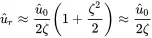(1.50)

with the corresponding phase angle

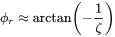(1.51)

The amplitude- and phase resonances are assumed to be equal for systems with small damping. The magnification is thus 1/2ζ, and it is called the quality factor:

(1.52)

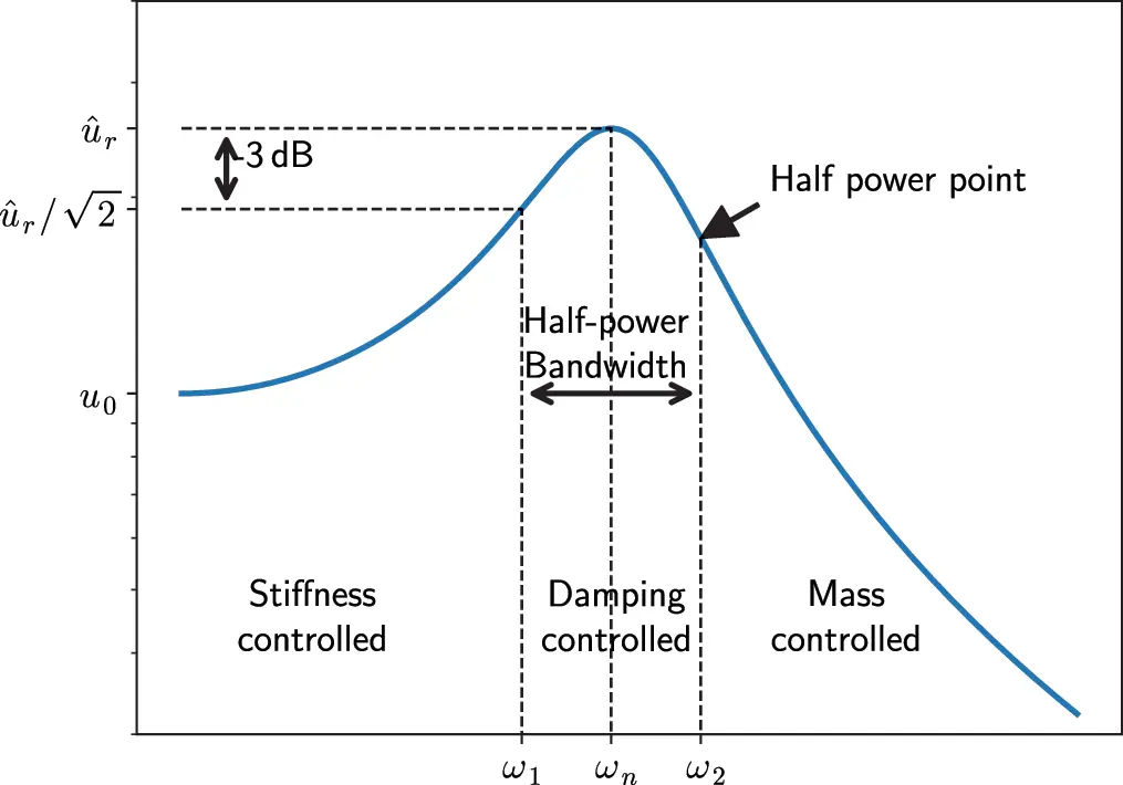
Figure 1.10Half power bandwidth for harmonic oscillator. Source : Alexander Peiffer.

This factor is a measure for the sharpness of the resonance peak or the quality of the resonator. In response diagrams when the shape of the amplitude over frequency is measured the half power bandwidth is used. This is the distance of the points where the amplitude is 1/2 of the peak value u^r. Solving Equation ( 1.31) for u^r/u^0=1/2 the frequencies of half power can be found:

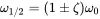(1.53)

and therefore

(1.54)

Obviously the decay time is also related to damping. If Equation ( 1.22) is considered we get

(1.55)

We have presented several expressions that describe damping. Nevertheless, even more quantities for damping are used depending on the engineering discipline and will be shown in Section 1.2.5. Section 1.2.5.1 aims at sorting all those expressions and their relationships among each other.

Viscous damping is rare in real systems, it only exists if the surface that is connected to liquids moves so slow that no turbulent motion appears. Observation of experiments with damping normally doesn’t show damping that increases with frequency as would be the case with viscous damping. Examples for damping processes are:

structural or hysteretic damping

coulomb or dry-friction damping

velocity-squared or aerodynamic drag damping.

As most systems are lightly damped so that damping can be neglected except near resonance, it is sufficient to approximate the non-viscous damping in terms of equivalent viscous damping. A good way to formulate a criteria that works for all types of damping is to consider the dissipated energy per cycle of vibration. For viscous damping this reads as

With the dissipated energy per cycle ΔEcycle for any particular damping type the equivalent viscous damping cveq can be determined from

(1.56)

In many cases damping is caused by structural damping. If materials like aluminium or steel are cyclically stressed they form a hysteresis loop. Experimental observations show, that the energy dissipated per cycle is proportional to the square of the strain (displacement):

(1.57)

Comparing this with Equation ( 1.56) gives:

(1.58)

Entering this into the equation of motion in complex form ( 1.27)

(1.59)

and rewriting ( 1.59) leads to

(1.60)

with the structural loss factor

(1.61)

and

(1.62)

In this case the displacement response reads:

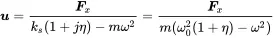(1.63)

The structural loss factor is of great importance for structural dynamics not only because of the frequent occurrence in practical systems but also for numerical methods. The equation of motion remains similar to the equation for undamped systems. Additionally, the frequency of structurally damped systems does not change. This can be seen if the equivalent viscous damping of structurally damped systems is introduced in the solution for the magnification factor and the phase: