Alexander Peiffer - Vibroacoustic Simulation

In most cases the life of an acoustic engineer means solving the target conflict between the acoustic performance and costs, weight, and space requirements. This is the reason why design engineers are not always the best friends of acousticians during the design phase. The more important it is that you are able to calculate the effect of your decisions for efficient application of the sometimes rare acoustic resources. I hope that this book provides some support for this demanding task.

Coming back to my initial motivation: If I would have to hold a lecture on vibroacoustic simulation now, I would sleep much better.

Alexander Peiffer

Planegg, Germany

15 October 2021

Special thanks goes to my former colleague Ulf Orrenius who wrote the train- and motivation section of chapter 12. His great experience and knowledge strongly enriched the content of this chapter.

I would also like to thank the Audi AG who provided the models to present the simulation strategy of automotive systems.

2DOFTwo degrees of freedom msMean square rmsRoot mean square CFDComputational fluid dynamics CFRPCarbon fiber reinforced plastic DFTDiscrete Fourier transform DVADynamic vibration absorber DOFDegree of freedom EMAExperimental modal analysis FEMFinite element method FFTFast Fourier transform FTFourier transform GFRPGlass fiber reinforced plastic HVACHeating, ventilation, and air conditioning MACModal assurance criterion MDOFMultiple degrees of freedom MIMOMultiple input multiple output NVHNoise, vibration, and harshnes PAXPassenger SDOFSingle degree of freedom SEAStatistical Energy Analysis SISOSingle input single output TBLTurbulent boundary layer TPATransfer path analysis TVATuned vibration absorber

Simple systems with properties constructed by lumped elements as masses, springs and dampers are a good playground to understand and investigate the physics of dynamic systems. Many phenomena of vibration as resonance, forced vibration and even first means of vibration control can be explained and visualized by these lumped systems.

In addition, a basic knowledge of signal and system analysis is required to put the principle of cause and effect in the right context. Every vibroacoustic system response depends on excitation by random, harmonic or specific signals in the time domain and we need a mathematical tool set to describe this.

An excellent test case to demonstrate and define the principle effects of vibration is the harmonic oscillator. It consists of a point mass, a spring and a damper. The combination of many point masses connected via simple springs and dampers provides some further insight into dynamic systems.

As those systems are described by components that have no dynamics in themselves they are called lumped systems. In principle all vibroacoustic systems can by modelled and approximated by this simplified approach.

A realization of the harmonic oscillator is given by a concentrated point mass m fixed at massless spring with stiffness k sas in Figure 1.1. The static equilibrium is assumed at u = 0 being the displacement in x -direction. A damper connecting mass and fixation creates dissipation.

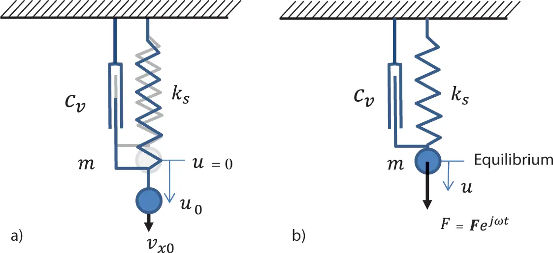
Figure 1.1 Damped harmonic oscillator with initial conditions a) and external force excitation b). Source : Alexander Peiffer.

Without external excitation as shown in Figure 1.1 a) the motion depends on the initial conditions at time t = 0 with the displacement u(0)=u0 and velocity vx(0)=vx0. The damping is supposed to be viscous, thus proportional to the velocity Fxv=−cvu˙. The equation of motion

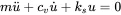(1.1)

is a homogeneous second order equation with a solution of the form u=Aest. Entering this into Equation ( 1.1) leads to the characteristic equation

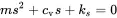(1.2)

with the two solutions

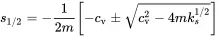(1.3)

Hence,

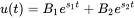(1.4)

with B 1and B 2depending on the initial conditions. The root in Equation ( 1.3) is zero when c vequals 4mks. This specific value is called the critical viscous damping damping

(1.5)

We use the following definitions:

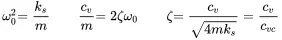(1.6)

ω 0is the natural angular frequency, ζ is ratio of the viscous-damping to the critical viscous-damping. There are additional expressions for the period and frequency

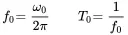(1.7)

where f 0is the natural frequency and T 0the oscillation period. Equations ( 1.1)–( 1.3) can now be written as

(1.8)

(1.9)

(1.10)

The problem falls into three cases:

ζ > 1 overdamped

ζ < 1 underdamped

ζ = 1 critically damped.

The first case leads to two real roots, and no oscillation is possible. The second case gives two complex roots, which means that (damped) oscillation occurs. The third case is a transition case between the two other. Subsections 1.1.2–1.1.4 deal with each case in detail.

Both roots in Equation ( 1.10) are real, distinct and negative. The motion is called overdamped because introducing this into Equation ( 1.4) gives a sum of decaying exponential functions:

(1.11)