Alexander Peiffer - Vibroacoustic Simulation

(1.30)

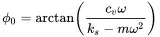
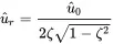
At ω = 0 the static displacement amplitude is u^0=F^x/ks. Using the definitions from ( 1.6) and dividing u^ by u^0 gives the normalized amplitude

(1.31)

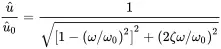
and phase

(1.32)

It can be shown that the maximum of u^ is at

(1.33)

and the maximum value is

(1.34)

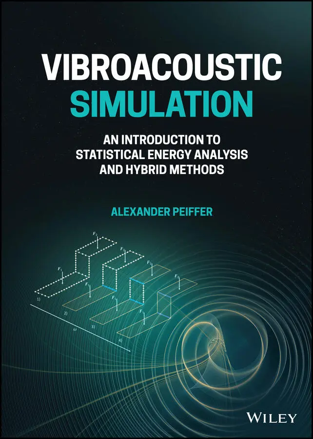
with the corresponding phase

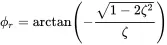(1.35)

The evolution of u^/u^0 and ϕ 0is shown in Figures 1.6 and 1.7 for different ζ . One can see the resonance amplification at ω rthat would be infinite in case of ζ = 0 and the decrease of the amplitude with increasing damping. For ζ>1/2 the maximum value occurs at ω = 0, so the displacement is just a forced movement without any resonance effect.

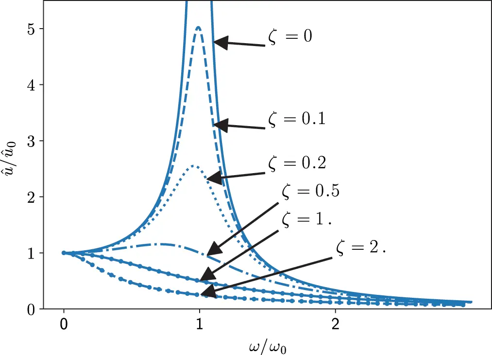
Figure 1.6 Normalized amplitude of forced harmonic oscillator. Source : Alexander Peiffer.

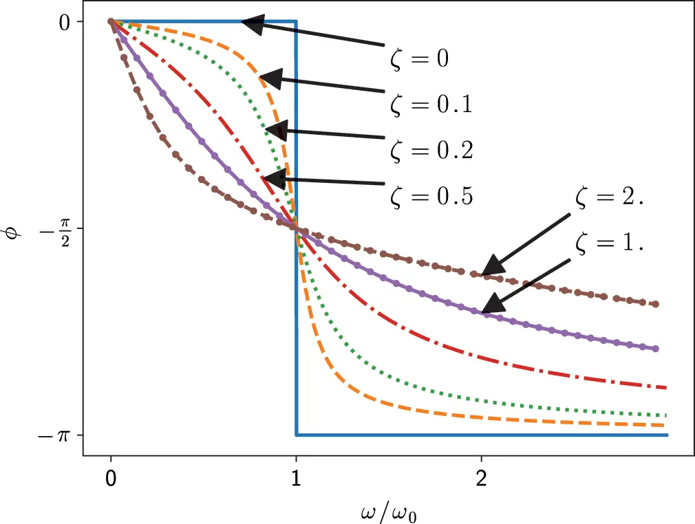
Figure 1.7 Phase of forced harmonic oscillator. Source : Alexander Peiffer.

The frequency of highest amplitude is called the amplitude resonance and it is different from the so called phase resonance with ϕ=−π2, which corresponds to the resonance of the undamped oscillator.

It is helpful to investigate the ongoing processes from the energy perspective. For an undamped system cv=0 that oscillates with u(t)=u^cos⁡(ω0t) and absence of external forces the energy remains constant. The energy is the sum of kinetic E kinand potential energy E pot

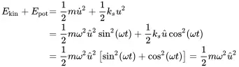(1.36)

and is constant, but spring and mass exchange energy twice over one period T 0.

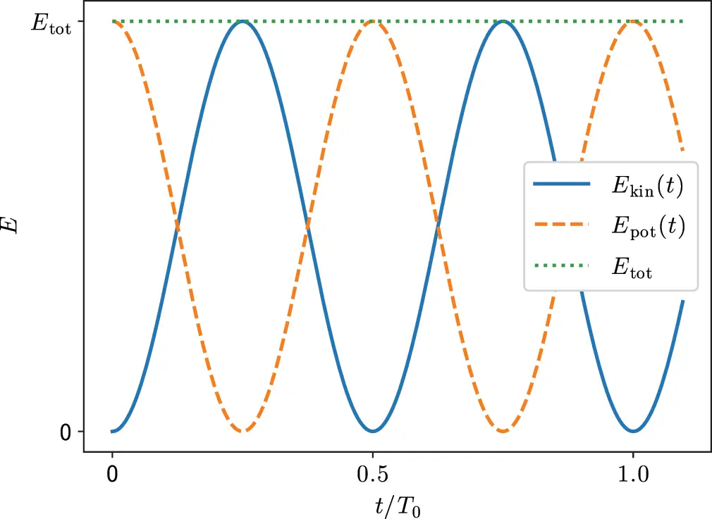
Figure 1.8Kinetic and potential energy of the harmonic oscillator. Source : Alexander Peiffer.

As energy quantities are not always constant, this motivates the definition of time average values. average ! time We introduce the mean-square (ms) and root-mean-square (rms) value for the time average for an arbitrary signal x ( t ). The mean-square value over a time T is

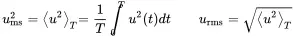(1.37)

In the following ⟨⋅⟩T=1T∫0T⋅dt denotes a time average. If the signal is harmonic with u(t)=u^cos⁡(ω0t) then

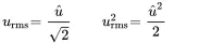(1.38)

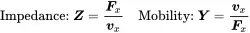
So far the frequency response of the oscillator was expressed as the relationship between displacement and force. The ratios u/Fx and D=Fx/u are called mechanical receptance and, respectively. Often used force response relationships are the mechanical impedance impedance ! mechanical (force/velocity=Fx/vx) and the mobility (velocity/force=vx/Fx). The symbols and definitions are:

(1.39)

Considering the solution of the damped oscillator and vx=jωu both quantities become:

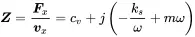(1.40)

The real and imaginary part have specific names resistance reactance

(1.41)

The meaning of this convention becomes clear when inspecting Figure 1.9. When the oscillator is excited in the mass- or stiffness-controlled regime below or above the resonance, the force introduces a reactive movement. The energy can be taken back from the system and it is called reactive . Whether the system response is mass or stiffness controlled can be identified from the slope of the impedance magnitude and the phase. In the resonance regime the system is driven at resonance and the damper dissipates energy. The resistance of the system becomes important and is thus called resistive .

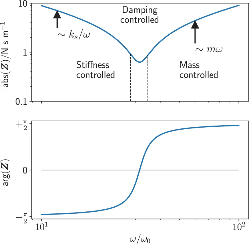
Figure 1.9 Magnitude and phase of oscillator impedance. Source : Alexander Peiffer.

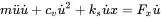
We multiply Equation ( 1.23) by u˙

(1.42)

The first and third term can be integrated

(1.43)

The terms in the parenthesis are kinetic and potential energy and known as constant. The expression cvu˙2 is the dissipated power, because it is the damping force times velocity.

(1.44)

And Fxu˙ is the introduced power, thus

(1.45)

So we get the power balance

(1.46)