Alexander Peiffer - Vibroacoustic Simulation
Здесь есть возможность читать онлайн «Alexander Peiffer - Vibroacoustic Simulation» — ознакомительный отрывок электронной книги совершенно бесплатно, а после прочтения отрывка купить полную версию. В некоторых случаях можно слушать аудио, скачать через торрент в формате fb2 и присутствует краткое содержание. Жанр: unrecognised, на английском языке. Описание произведения, (предисловие) а так же отзывы посетителей доступны на портале библиотеки ЛибКат.
- Название:Vibroacoustic Simulation
- Автор:
- Жанр:
- Год:неизвестен
- ISBN:нет данных
- Рейтинг книги:3 / 5. Голосов: 1
-
Избранное:Добавить в избранное
- Отзывы:
-
Ваша оценка:
Vibroacoustic Simulation: краткое содержание, описание и аннотация
Предлагаем к чтению аннотацию, описание, краткое содержание или предисловие (зависит от того, что написал сам автор книги «Vibroacoustic Simulation»). Если вы не нашли необходимую информацию о книге — напишите в комментариях, мы постараемся отыскать её.
Learn to master the full range of vibroacoustic simulation using both SEA and hybrid FEM/SEA methods Vibroacoustic Simulation
Vibroacoustic Simulation
Vibroacoustic Simulation
Vibroacoustic Simulation — читать онлайн ознакомительный отрывок
Ниже представлен текст книги, разбитый по страницам. Система сохранения места последней прочитанной страницы, позволяет с удобством читать онлайн бесплатно книгу «Vibroacoustic Simulation», без необходимости каждый раз заново искать на чём Вы остановились. Поставьте закладку, и сможете в любой момент перейти на страницу, на которой закончили чтение.
Интервал:
Закладка:
The movement of such a system is illustrated in Figure 1.2. Using the above solution and applying the initial conditions u 0and vx0 we get for B i:
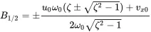 (1.12)
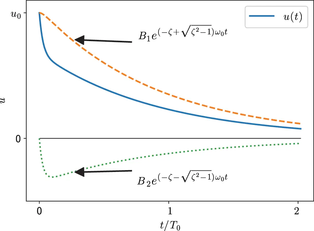
Figure 1.2 Decaying components of the overdamped oscillator. Source : Alexander Peiffer.
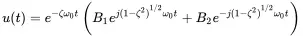
1.1.3 The Underdamped Oscillator (ζ < 1)
Here, the roots are complex conjugates and the solution of Equation ( 1.10) becomes:
 (1.13)
 (1.14)
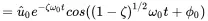
The motion is oscillatory with a frequency that is lower than in the undamped configuration:
 (1.15)
Introducing the initial conditions u 0and vx0 at t = 0 the solution for the initial amplitude u^0 and phase ϕ 0reads as:
 (1.16)
 (1.17)
The damped oscillatory motion is illustrated in Figure 1.3. It shows a decreasing motion that never approaches the equilibrium.

Figure 1.3 Damped, sinusoidal motion of the underdamped oscillator. Source : Alexander Peiffer.
1.1.4 The Critically Damped Oscillator (ζ = 1)
The last case is a transition between both systems. There is only one root s=−ω0, and the solution in Equation ( 1.4) becomes:
 (1.18)
This solution does not provide enough constants to fulfil the initial conditions, so that we need an extra term te−ω0t:
 (1.19)
Introducing the initial conditions again, the constants are:
 (1.20)
 (1.21)
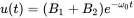
Critically damped systems can be of practical relevance, because the motion returns to rest in the shortest possible time, which is useful if periodic motion shall be prevented. In contrast to the overdamped oscillator the equilibrium is reached as can be seen in Figure 1.4.
Figure 1.4 Motion of the critically damped oscillator. Source : Alexander Peiffer.
Let us summarize some facts and observations about free damped oscillators:
1 Oscillation occurs only if the system is underdamped.
2 ωd is always less than ω0.
3 The motion will decay.
4 The frequency ωd and the decay rate are properties of the system and independent from the initial conditions.
5 The amplitude of the damped oscillator is u^(t)=u^0e−βt with β=ζω0. β is called the decay rate of the damped oscillator.
The decay rate is related to the decay time τ . This is the time interval where the amplitude decreases to e−1 of the initial amplitude. Thus, the decay time is:
 (1.22)
1.2 Forced Harmonic Oscillator
When an external force F^xcos(ωt) is exciting the damped oscillator as shown in Figure 1.1 b), applying Newton’s second law we get for the equation of motion:
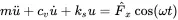 (1.23)
This is an inhomogeneous, linear, second-order equation for u . The solution of this equation is given by a particular solution uP(t) and the solutions of the homogeneous Equation ( 1.1) uH(t).
 (1.24)
Any linear combination of the homogeneous solution can be added to the particular solution because it equals zero.
1.2.1 Frequency Response
There are several methods to determine the particular solutions, like Laplace and Fourier transforms. Here, complex algebra will be used 1. Amplitude and phase are given by a complex pointer denoted by bold italic type as depicted in Figure 1.5.
 (1.25)
Figure 1.5 Complex pointer, amplitude and phase relationship. Source : Alexander Peiffer.
F xis the complex amplitude of the force, and the Re(⋅) expression is usually omitted. The displacement and velocity response is then given by
 (1.26)
with uand v xas complex amplitudes of the displacement and velocity, respectively. Introducing this into Equation ( 1.23).
 (1.27)
and solving this for ugives:
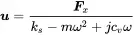 (1.28)
The magnitude u^ and the phase ϕ of uare:
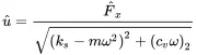 (1.29)
Интервал:
Закладка:
Похожие книги на «Vibroacoustic Simulation»
Представляем Вашему вниманию похожие книги на «Vibroacoustic Simulation» списком для выбора. Мы отобрали схожую по названию и смыслу литературу в надежде предоставить читателям больше вариантов отыскать новые, интересные, ещё непрочитанные произведения.


Обсуждение, отзывы о книге «Vibroacoustic Simulation» и просто собственные мнения читателей. Оставьте ваши комментарии, напишите, что Вы думаете о произведении, его смысле или главных героях. Укажите что конкретно понравилось, а что нет, и почему Вы так считаете.