Alexander Peiffer - Vibroacoustic Simulation

(2.113)

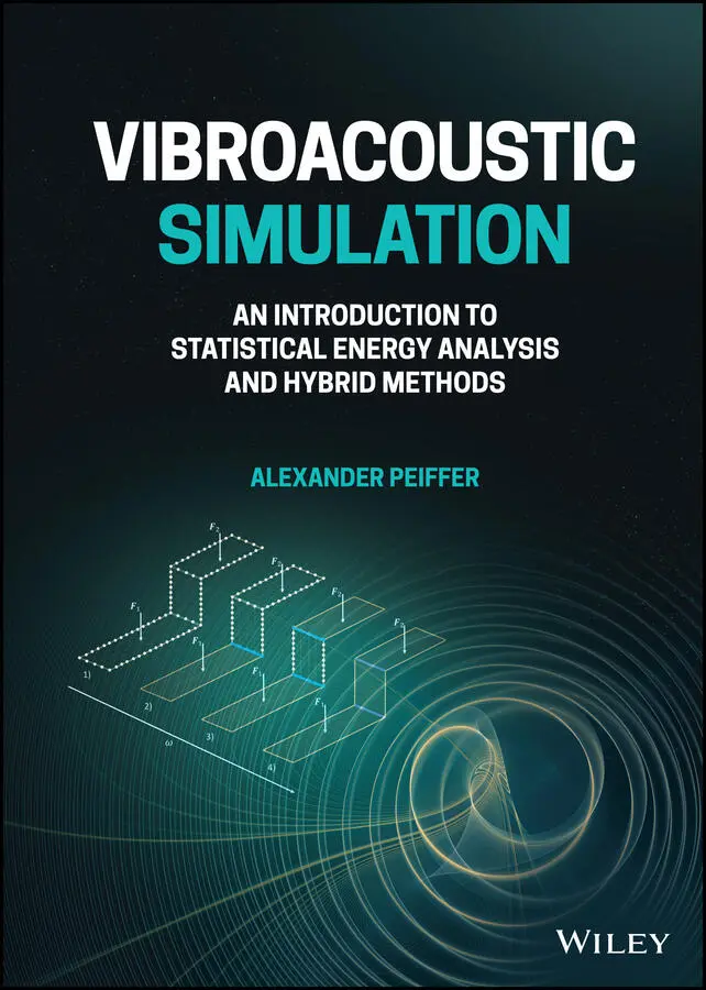
With these conditions we can factor out the exponential function

(2.114)

After clarifying the angles of reflection and transmission the next point is to assess the fraction of transmitted and reflected wave. From the continuity condition for the velocity in the z-direction we get with vz=−∂Φ/∂z when going through the algebra

(2.115)

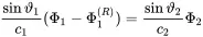
Rearranging equations ( 2.114) and ( 2.115) the reflection factor is

(2.116)

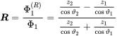
This expression is similar to ( 2.103) except the angle factor that represents the physics of the wave propagation in the second medium. The transmission factor is defined by the ratio of pressure amplitudes p1=jωρ1Φ1 and p2=jωρ2Φ2. Hence,

(2.117)

The transmitted acoustic power follows from the square of the amplitudes. We introduce a transmission coefficient τ by

(2.118)

Without loss of generality we assume ϑ=0 so each power is given by

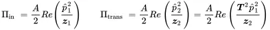
With ( 2.117) this reads as:

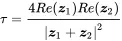(2.120)

It should be noted that the transmission coefficient of the flat interface between two fluids is determined by the impedance of each half space ‘seen’ from the other side. This is the first indication for the coupling of subsystems determined by the radiation impedance into the free fields of each subsystem. Similar expressions will be found in Sec. 8.2.4.1 when transmission is dealt with in the context of coupled random subsystems.

In the considerations in this chapter so far, we neglected the source terms related to the conservation of mass and momentum. All sources discussed until now are caused by vibrating surfaces. For establishing a physical link between the source term and the specific mass flow q˙s in Equation ( 2.3) and force density term f in Equation ( 2.8) we keep the terms this time. The source terms are not influenced by the linearization procedure; thus, the inhomogeneous and linear equations of momentum ( 2.24) and continuity ( 2.23) read as

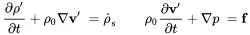(2.121)

Repeating the steps of section 2.2.5 we finally get the inhomogeneous wave equation

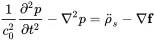(2.122)

The density source is converted into a volume source strength density by ρ˙s=ρ0qs(t). The above equation can also be converted into the frequency domain and hence to the inhomogeneous Helmholtz equation

(2.123)

This section presents the concept of the Green’s function that uses a formalism to calculate the sound field for arbitrary source and boundary configurations as shown for example by Morse and Ingard (1968).

The Green’s function is defined as the solution of the following inhomogeneous wave equation.

(2.124)

The inhomogeneous part is the delta function which allows for this elegant derivation of the Kirchhoff integral. The delta function is introduced in the appendix A.1.3 in the time domain. However, it can also be applied in space. The multidimensional delta function is simply the product of three Dirac delta functions in space

(2.125)

The sifting properties and the value of the integration is defined by volume integral

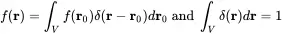(2.126)

The solution of Equation ( 2.124) is the point source ( 2.91) 3.

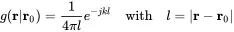(2.127)

In order to achieve a common formulation we add an arbitrary solution χ of the homogeneous wave equation

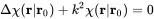(2.128)

to the Green’s function to get the generalized Green’s function

(2.129)

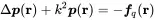
The purpose of the additional homogeneous solution is to create freedom to fulfill boundary conditions that do not occur in the free sound field. The task is to find the solution for the inhomogeneous wave equation

(2.130)

The generalized Green’s function must be a solution of the following equation for the special case with r,r0∈V and the boundary ∂V as shown in Figure 2.9.

(2.131)

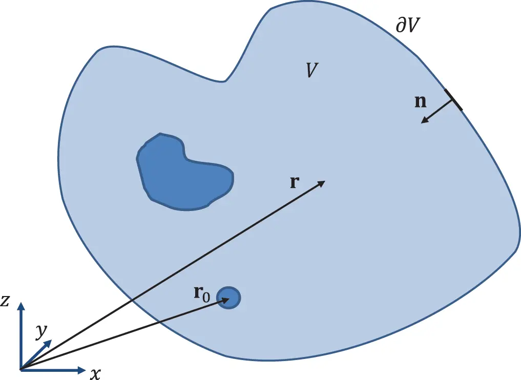
Figure 2.9 Solution volume and boundaries. Source : Alexander Peiffer.

In order to receive a global solution we perform the operation

(2.132)

This leads to

(2.133)