Alexander Peiffer - Vibroacoustic Simulation

With the D’Alambert solution for spherical waves ( 2.66) we can also derive a point source in time domain

(2.93)

The point source is of great importance for the solution of the inhomogeneous wave equation in combination with complex boundary conditions. Any source can be reconstructed by a superposition of point sources as shown in Section 2.7.

Performing the limit process with kR→0 and taking the power from equation 2.86we get the intensity of the point source:

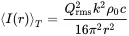(2.94)

and the total radiated power

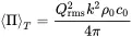(2.95)

with radiation impedance following from this

(2.96)

A plane wave striking a plane surface is a first example of interaction with obstacles. Imagine a configuration as shown in Figure 2.7. The impedance of the surface is z2, and it is given by using the velocity vz perpendicular to the plane.

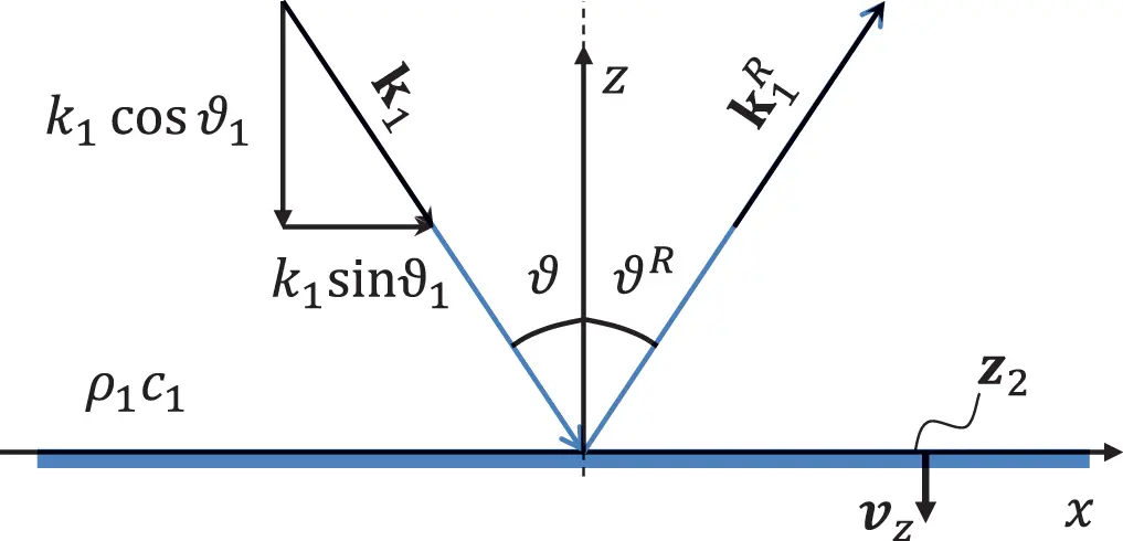
Figure 2.7 Reflection of a plane wave at an infinite surface with impedance Z2. Source : Alexander Peiffer.

Without loss of generality the wave front is parallel to the y-axis and all properties are functions of x and z. The solution in the half space of z>0 is the superposition of two plane waves.

(2.97)

With the following arguments of the exponential function

(2.98)

(2.99)

The pressure at the surface z=0 is given by

(2.100)

and the velocity in z-direction reads

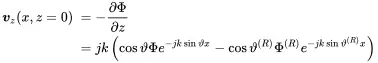(2.101)

We certainly shall not be able to match the impedance z2=p/vz at every surface position unless the arguments of the exponential functions are equal, hence

So, we get from the surface impedance condition

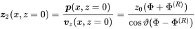(2.102)

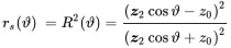
With z0=ρ0c0 and rearranging the above equation, the reflection factor is given by

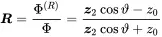(2.103)

The ratio between irradiated power to reflector power is the squared reflection factor called the.

(2.104)

(2.105)

Note that those coefficients are exclusively described by the impedance of fluid and surface and not density or speed of sound. Thus, the impedance is the relevant quantity here.

A plane wave passing a flat interface between two infinite fluid volumes with different density and sound velocity as shown in Figure 2.8 is a first example of continuous systems exchanging acoustic energy. Applications of such a system could be for example the interface between a liquid (water) and a gas (air) or just different gases.

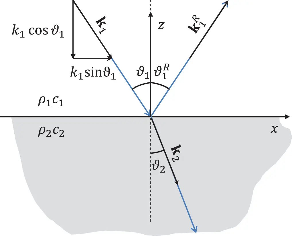
Figure 2.8 Transmission and reflection of a plane wave at the interface of two fluids. Source : Alexander Peiffer.

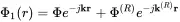
Region 1 of the incoming wave has two wave components, the incoming and the reflected wave, and region 2 the transmitted wave. Thus, both velocity potentials read

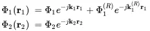(2.106)

Using the given angles as sketched in Figure 2.8 the wavenumber space vector products are given by

(2.107)

(2.108)

(2.109)

with k1=ω/c1 and k2=ω/c2. The contact face between the fluid requires the continuity of pressure and velocity in the z-direction. We start with the pressure p1/2=jωρ1/2Φ1/2. Entering equations ( 2.107)–( 2.109) into (2.106) and determining the pressure relation

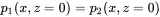
gives

(2.110)

A solution for any x is only possible if the arguments of the exponential functions are equal.

(2.111)

So also in the transmission case the incident angle equals the angle of the reflected wave. Additionally we have

(2.112)

This represents the acoustic equivalent of Snell’s law of transmission: