James W. Brown - Principles of Microbial Diversity
Здесь есть возможность читать онлайн «James W. Brown - Principles of Microbial Diversity» — ознакомительный отрывок электронной книги совершенно бесплатно, а после прочтения отрывка купить полную версию. В некоторых случаях можно слушать аудио, скачать через торрент в формате fb2 и присутствует краткое содержание. Жанр: unrecognised, на английском языке. Описание произведения, (предисловие) а так же отзывы посетителей доступны на портале библиотеки ЛибКат.
- Название:Principles of Microbial Diversity
- Автор:
- Жанр:
- Год:неизвестен
- ISBN:нет данных
- Рейтинг книги:5 / 5. Голосов: 1
-
Избранное:Добавить в избранное
- Отзывы:
-
Ваша оценка:
Principles of Microbial Diversity: краткое содержание, описание и аннотация
Предлагаем к чтению аннотацию, описание, краткое содержание или предисловие (зависит от того, что написал сам автор книги «Principles of Microbial Diversity»). Если вы не нашли необходимую информацию о книге — напишите в комментариях, мы постараемся отыскать её.
provides a solid curriculum for students to explore the enormous range of biological diversity in the microbial world. Within these richly illustrated pages, author and professor James W. Brown provides a practical guide to microbial diversity from a phylogenetic perspective in which students learn to construct and interpret evolutionary trees from DNA sequences. He then offers a survey of the «tree of life» that establishes the necessary basic knowledge about the microbial world. Finally, the author draws the student's attention to the universe of microbial diversity with focused studies of the contributions that specific organisms make to the ecosystem.
Principles of Microbial Diversity
Principles of Microbial Diversity — читать онлайн ознакомительный отрывок
Ниже представлен текст книги, разбитый по страницам. Система сохранения места последней прочитанной страницы, позволяет с удобством читать онлайн бесплатно книгу «Principles of Microbial Diversity», без необходимости каждый раз заново искать на чём Вы остановились. Поставьте закладку, и сможете в любой момент перейти на страницу, на которой закончили чтение.
Интервал:
Закладка:
Long-branch attraction
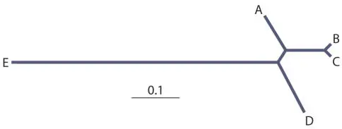
One of the things substitution models fight is a treeing artifact called long-branch attraction. Long-branch attraction is the result (primarily) of an underestimation of the evolutionary distance of distantly related sequences. This underestimation results in a tendency for the longest branches in a tree to artificially cluster together; this also results in the artificial clustering of short branches. Figure 5.4 shows a very simple demonstration of how long-branch attraction can result in incorrect trees.
Long-branch attraction happens because of the difference in evolutionary rates in the branches. Therefore, it is always worth worrying about the details of trees containing branches with very different evolutionary rates, i.e., those with branches of very different lengths.
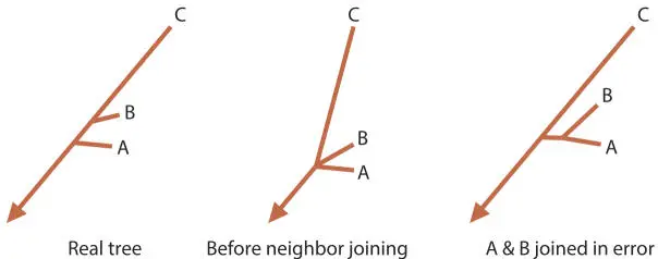
Figure 5.4Generation of a “long-branch attraction” artifact in a phylogenetic tree. If the sub-tree to the left is the representation of how these sequences are actually related, imagine what would happen in a neighbor-joining analysis. Sequences A and B are more alike (i.e., they have a smaller evolutionary distance between them) than either is to C, and so they will be erroneously joined, as shown on the right. doi:10.1128/9781555818517.ch5.f5.4
One of the primary causes of strikingly long branches, by the way, is bad sequence or poor alignment. If the primary sequence data are poor, every mistake in the data will be counted as an evolutionary change by the treeing algorithm. Likewise, poor alignment causes most of the bases in the poorly aligned region to be counted as evolutionary changes, lengthening the branch leading to that sequence. Again, beware of trees with unexpectedly long branches! Poor alignment or bad sequence data, resulting in long branches, can combine with long-branch attraction to make trees meaningless.
Treeing algorithms
Fitch-Margoliash: an alternative distance-matrix treeing method
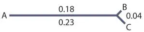
Another useful method for generating trees from distance matrices is that of Fitch and Margoliash, commonly called Fitch. This algorithm starts with two of the sequences, separated by a line equal to the length of the evolutionary distance between them. For example, for this distance matrix:
| Evolutionary distance | |||||
| A | B | C | D | E | |
| A | — | — | — | — | — |
| B | 0.18 | — | — | — | — |
| C | 0.23 | 0.04 | — | — | — |
| D | 0.29 | 0.35 | 0.29 | — | — |
| E | 0.77 | 0.77 | 0.77 | 0.77 | — |
one might start with sequences A and B (usually in practice, the sequences are chosen randomly):

Then the next sequence is added to the tree such that the distances between A, B, and C are approximately equal to the evolutionary distances:
Note that the fit is not perfect. If we could determine the evolutionary distances exactly, they would fit the tree exactly, but since we have to estimate these distances, the numbers are fit to the tree as closely as possible using averaging or least-squares best fit.
The next step is to add the next sequence, again readjusting the tree to fit the distances as well as possible:
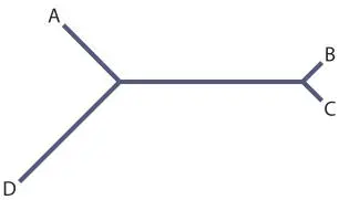
And at last we can add the final sequence and readjust the branch lengths one last time using least-squares:
Neighbor joining and Fitch are both least-squares distance-matrix methods, but a big difference is that neighbor joining separates the determination of the tree structure from solving branch lengths, whereas Fitch solves them together but does so by adding branches (sequences) one at a time.
Parsimony
Parsimony is actually a collection of related methods based on the premise of Occam’s razor. In other words, the tree that requires the smallest number of sequence changes to generate the sequences in the alignment is the most likely tree.
For example:
No distance matrix is calculated; instead, trees are searched and each ancestral sequence is calculated, allowing for all uncertainties, in a process analogous to Sudoku puzzles. The number of “mutations” required is added up, and the tree with the best score wins. Testing every possible tree is not usually possible (the number of trees grows exponentially with the number of sequences), so a variety of search algorithms are used to examine only the most likely trees. Likewise, there are a variety of ways of counting (scoring) sequence changes.
Parsimony methods are typically slower than distance-matrix methods but very much faster than the maximum-likelihood methods described below. Parsimony uses more of the information in an alignment, since it does not reduce all of the individual sequence differences to a distance matrix, but it seems to work best with relatively closely related sequences and is not usually used for rRNA sequences.
Maximum likelihood
The maximum-likelihood method turns the tree construction process on its head, starting with a cluster analysis to generate a “guide” tree, from which a very complete substitution model is calculated. The algorithm then goes back and calculates the likelihood of any particular tree by summing the probabilities of all of the possible intermediates required to get to the observed sequences. Rather than try to calculate this for all possible trees, a heuristic search is used starting with the guide tree. Sound complicated? It is, and maximum-likelihood tree construction is by far the most computationally intensive of the methods in common use. However, it is generally also the best, in the sense that the trees are more consistent and robust. The limitation is that fewer and shorter sequences can be analyzed by the maximum-likelihood method because of its computational demands. A tree that might take a few seconds by neighbor joining or a few minutes by parsimony or Fitch can take a few hours or a couple of days by maximum likelihood. This is serious; it means that you cannot usually “play” with trees, testing various changes in the data or treeing parameters and seeing the result immediately.
Bayesian inference
Bayesian inference is a relatively new approach to tree construction. This approach starts with a random tree structure, random branch lengths, and random substitution parameters for an alignment, and the probability of the tree being generated from the alignment with these parameters is scored. Obviously the initial score is likely to be very poor. Then a random change is made in this tree (branch order, branch length, or substitution parameter) and the result is rescored. Then a choice is made whether to accept the change; this choice is partially random, but the greater the improvement in tree score, the more likely it is to be accepted. If the change is accepted, the process is repeated starting with this new tree; if the change is rejected, the process is repeated starting with the old tree. After many, many cycles of this process, the algorithm settles in to a collection of trees that are nearly optimal. Various tricks are used to keep the algorithm from getting stuck in local-scoring minimum zones.
Читать дальшеИнтервал:
Закладка:
Похожие книги на «Principles of Microbial Diversity»
Представляем Вашему вниманию похожие книги на «Principles of Microbial Diversity» списком для выбора. Мы отобрали схожую по названию и смыслу литературу в надежде предоставить читателям больше вариантов отыскать новые, интересные, ещё непрочитанные произведения.


Обсуждение, отзывы о книге «Principles of Microbial Diversity» и просто собственные мнения читателей. Оставьте ваши комментарии, напишите, что Вы думаете о произведении, его смысле или главных героях. Укажите что конкретно понравилось, а что нет, и почему Вы так считаете.